Daily Mediterranean 3D fields of temperature, salinity, sea water density, chlorophyll field and geostrophic current at 1/24° of resolution, up to 150m-depth and from 2016 to mid 2022.
Original Data Source: https://
4dmed .artov .ismar .cnr .it /thredds /catalog /4dmed /catalog _NN .html Reference: Sammartino & Buongiorno Nardelli (2024)
OSC entry: https://
opensciencedata .esa .int /products /4dmed -t -s -geo -a -150 /collection License: CC-BY-4.0
import xarray as xr

zarr_href = 'https://s3.waw4-1.cloudferro.com/EarthCODE/OSCAssets/4dmed/4dmed-bp.zarr/'
# this dataset is a geozarr (See the visualisation notebook for more information.)
ds = xr.open_zarr(zarr_href, group='0')
dsimport numpy as np
day_index = 15
surface_temp = (
ds['TEMP3D']
.isel(time=day_index)
.sel(depth=1, method="nearest")
.compute()
)
surface_tempimport matplotlib.pyplot as plt
import cartopy.crs as ccrs
import cartopy.feature as cfeature
# Set up the figure and the map projection
fig, ax = plt.subplots(figsize=(12, 8), subplot_kw={'projection': ccrs.PlateCarree()})
# Add geographic features for context
ax.add_feature(cfeature.COASTLINE, linewidth=0.8)
ax.add_feature(cfeature.LAND, facecolor='lightgray', zorder=100) # Put land on top of ocean
ax.add_feature(cfeature.BORDERS, linestyle=':', linewidth=0.5)
# 3. Plot filled contours (the colors)
filled_c = surface_temp.plot.contourf(
ax=ax,
x='lon',
y='lat',
transform=ccrs.PlateCarree(),
levels=20, # Number of color gradients
cmap='RdYlBu_r', # Red-Yellow-Blue colormap (reversed so red=warm)
cbar_kwargs={'label': 'Temperature (°C)'}
)
# plot contour lines on top
lines_c = surface_temp.plot.contour(
ax=ax,
x='lon',
y='lat',
transform=ccrs.PlateCarree(),
levels=20, # Keep levels identical to contourf to match boundaries
colors='black', # Black lines
linewidths=0.5,
alpha=0.5 # Slightly transparent
)
# Add a title dynamically using xarray attributes if they exist
time_str = str(surface_temp.time.values)[:10] # Gets 'YYYY-MM-DD'
ax.set_title(f"Mediterranean Sea Surface Temperature\nDate: {time_str}")
plt.show()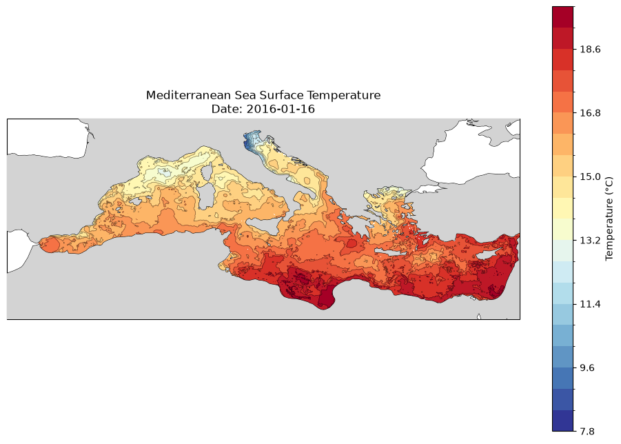
Visualisation
This dataset is in geozarr format, however it is not optimised for visualisaiton, but for analysis and therefore is chunked along the temporal and depth dimensions as well as spatially. Nevertheless, since the data is available at multiple resolutions it can be interactively visualised by any GeoZarr viewer by passing the dataset url. For example:
Through open-layers: https://
sunnydean .github .io /ocean _cubes _vis / ?cube = https:// s3 .waw4 -1 .cloudferro .com /EarthCODE /OSCAssets /4dmed /4dmed -bp .zarr/
See the visualisation section for more info.
- Sammartino, M., & Buongiorno Nardelli, B. (2024). ESA 4DMED-Sea - Neural network reconstruction of 3D Mediterranean bio-physical fields from surface observations at 1/24 deg. Istituto di Scienze Marine, Consiglio Nazionale delle Ricerche (ISMAR-CNR). 10.25423/CMCC/4DMEDSEA_BIOPHYS_REP_3D