Access Morlenn Mixed Layer Properties
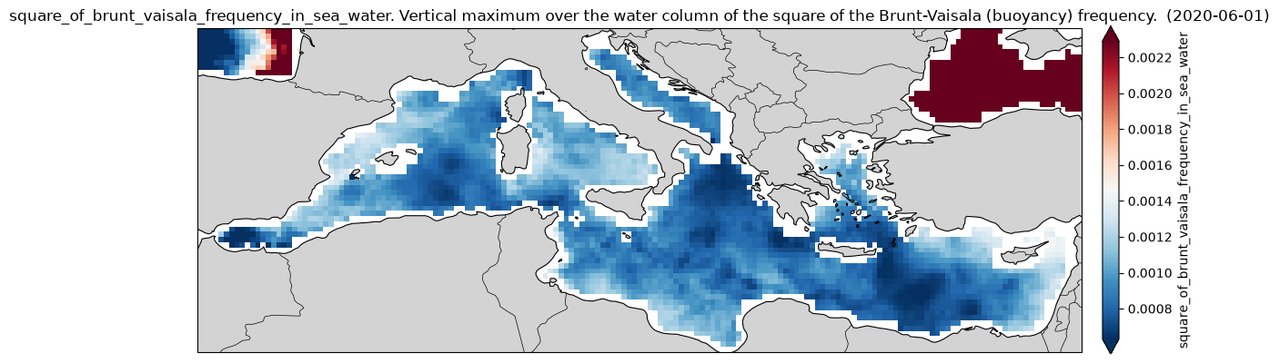
Mixed Layer Properties (MLD, N2max) reconstruction in the North Atlantic Ocean, Mediterranean sea and equatorial region using Morlenn algorithm, baseline and assim version within ESA UpperDyn project.
Original Data Source: https://
opensciencedata .esa .int /products /morlenn _mld /collection Reference: OceanDataLab (Lucile Gaultier, Parth Tripathi)
OSC entry: https://
opensciencedata .esa .int /products /morlenn _mld /collection License: CC-BY-4.0
import xarray as xrfrom pystac_client import Client
catalog = Client.open("https://eoapi.workspace.earthcode.eox.at/stac/")
collection = catalog.search(collections=["morlenn_mld"]).item_collection()
items = {item.id: item for item in collection}
collectionLoading...
[item.assets["data"].href for item in collection]Baseline model
ds = xr.open_zarr(items["morlenn_mld-morlenn_baseline"].assets["data"].href)
ds
Loading...
import cartopy.crs as ccrs
import cartopy.feature as cfeature

# Choose date
date = "2020-06-01"

# Select the air-sea CO2 flux for that date
n2 = ds["N2"].sel(
    longitude=slice(-6.062, 36.06),
    latitude=slice(30.27, 45.98),
)
n2 = n2.sel(time=date, drop=True, method="nearest")

n2
Loading...
# use the xarray plotting interface to create a map
img = n2.plot.imshow(
    subplot_kws={"projection": ccrs.PlateCarree()},
    transform=ccrs.PlateCarree(),
    size=4,
    aspect=3,
    robust=True,
    cmap="RdBu_r",
    cbar_kwargs={"label": "square_of_brunt_vaisala_frequency_in_sea_water", "pad": 0.02},
)

fig, ax = img.figure, img.axes

ax.add_feature(cfeature.LAND, facecolor="lightgray")
ax.add_feature(cfeature.COASTLINE, linewidth=0.8)
ax.add_feature(cfeature.BORDERS, linewidth=0.5)

ax.set_title(f"square_of_brunt_vaisala_frequency_in_sea_water. Vertical maximum over the water column of the square of the Brunt-Vaisala (buoyancy) frequency.  ({date})")

fig.tight_layout()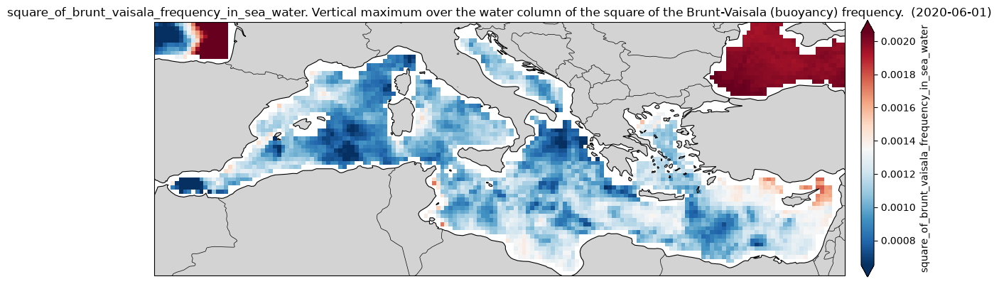
Assim Model
ds = xr.open_zarr(items["morlenn_mld-morlenn_assim"].assets["data"].href)
ds
Loading...
# Choose date
date = "2020-06-01"

# Select the air-sea CO2 flux for that date
n2 = ds["N2"].sel(
    longitude=slice(-6.062, 36.06),
    latitude=slice(30.27, 45.98),
)
n2 = n2.sel(time=date, drop=True, method="nearest")

n2
Loading...
# use the xarray plotting interface to create a map
img = n2.plot.imshow(
    subplot_kws={"projection": ccrs.PlateCarree()},
    transform=ccrs.PlateCarree(),
    size=4,
    aspect=3,
    robust=True,
    cmap="RdBu_r",
    cbar_kwargs={"label": "square_of_brunt_vaisala_frequency_in_sea_water", "pad": 0.02},
)

fig, ax = img.figure, img.axes

ax.add_feature(cfeature.LAND, facecolor="lightgray")
ax.add_feature(cfeature.COASTLINE, linewidth=0.8)
ax.add_feature(cfeature.BORDERS, linewidth=0.5)

ax.set_title(f"square_of_brunt_vaisala_frequency_in_sea_water. Vertical maximum over the water column of the square of the Brunt-Vaisala (buoyancy) frequency.  ({date})")

fig.tight_layout()