Explore re-projected dataset in the Med cube
This database contains the two Ocean-Soda datasets - v1 and v2, which are different products on different temporal scales and grids.
ocean-soda.zarr - a global monthly gridded dataset of the surface ocean carbonate system for seasonal to decadal studies of ocean acidification. The result of ocean soda v1.
OceanSODA_ETHZv2.r2026.GCB-fgco2-1982_2025-pyramid.zarr - which is a geozarr of a global 8day gridded dataset of the surface ocean carbonate system . The result of ocean soda v2.
OceanSoda v2 (2025) an older version of the above dataset.
Original Data Source: Gregor, Luke & Gruber, Nicolas (2020)
Reference: Gregor, Luke & Gruber, Nicolas (2020)
OSC entry: https://
opensciencedata .esa .int /products /ocean -soda -ethz /collection License: CC-BY-NC-SA-4.0
OceanSoda v2
import pandas as pd
import xarray as xr
from pystac_client import Client

catalog = Client.open("https://eoapi.workspace.earthcode.eox.at/stac/")
collection = catalog.search(collections=["oceansoda-ethz-v2", "ocean-soda-ethz"]).item_collection()
items = {item.id: item for item in collection}
collection[item.assets["data"].href for item in collection]ds_v2 = xr.open_zarr(items["OceanSODA_ETHZv2.r2026.GCB-fgco2-1982_2025-pyramid"].assets["data"].href, group='0') # read the first group, this is the highest resolution available data
ds_v2import cartopy.crs as ccrs
import cartopy.feature as cfeature
# Choose date
date = "2020-06-01"
# Select the air-sea CO2 flux for that date
pp = ds_v2["fgco2"].sel(
lon=slice(-6.062, 36.06),
lat=slice(45.98, 30.27),
)
pp = pp.sel(time=date, drop=True, method="nearest")
# use the xarray plotting interface to create a map
img = pp.plot.imshow(
subplot_kws={"projection": ccrs.PlateCarree()},
transform=ccrs.PlateCarree(),
size=4,
aspect=3,
robust=True,
cmap="RdBu_r",
cbar_kwargs={"label": "Air-sea CO2 flux (mol m$^{-2}$ s$^{-1}$)\nBlue = uptake, Red = release", "pad": 0.02},
)
fig, ax = img.figure, img.axes
ax.add_feature(cfeature.LAND, facecolor="lightgray")
ax.add_feature(cfeature.COASTLINE, linewidth=0.8)
ax.add_feature(cfeature.BORDERS, linewidth=0.5)
ax.set_title(f"Air-sea CO2 flux between sea water and air ({date})")
fig.tight_layout()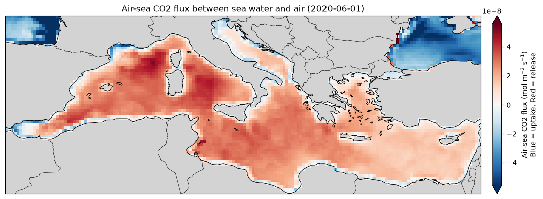
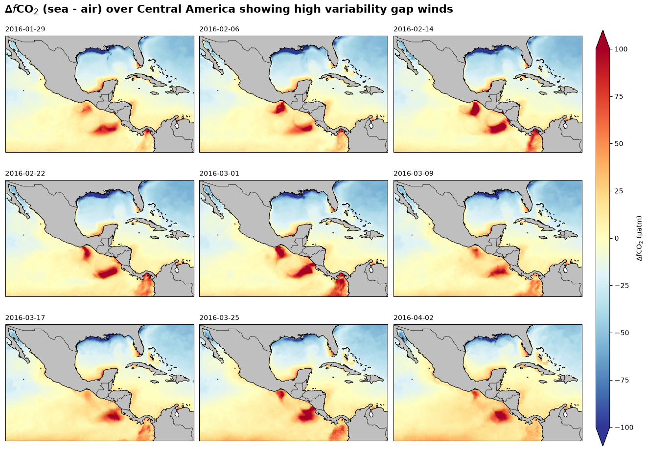
# calculate delta fco2 (sea - air)
dfco2 = ds_v2['sfco2'] - ds_v2['fco2atm']

# select a subset of the data for plotting (time series of maps)
da = dfco2.sel(
    lon=slice(-115.75, -67.28),
    lat=slice(33, 3),
    time=slice("2016-01-28", "2016-04-03"),
)

# plot using xarray's facet grid plotting interface
facet_grid = da.plot.imshow(
    subplot_kws={"projection": ccrs.PlateCarree()},
    transform=ccrs.PlateCarree(),
    aspect=1.5,
    size=3,
    col="time",
    col_wrap=3,
    vmin=-100, vmax=100,
    cmap="RdYlBu_r",
    cbar_kwargs={"label": "∆fCO$_2$ (µatm)", "pad": 0.02, "aspect": 30},
)


# fetch the figure and axes from the facet grid object
fig, axs = facet_grid.fig, facet_grid.axs.flatten()

# add basemap features to each subplot
for ax in axs:
    ax.add_feature(cfeature.LAND, facecolor="0.75")
    ax.add_feature(cfeature.COASTLINE, linewidth=0.8)
    ax.add_feature(cfeature.BORDERS, linewidth=0.5)

# adjusting titles
facet_grid.set_titles(template="", loc="center")
facet_grid.set_titles(template="{value}", loc="left")

fig.suptitle(
    "∆$f$CO$_2$ (sea - air) over Central America showing high variability gap winds",
    fontsize=16,
    x=0.01,
    y=1.02,
    ha="left",
    weight="bold",
)
OceanSODA v1
OceanSODA v1 also includes information about the ocean’s pH and other marine carbonate system paramters.
Here we look at how El Nino might impact pH estimates in the Eastern Equatorial Pacific
ds_v1 = xr.open_zarr(items["ocean-soda-zarr"].assets["data"].href, chunks={})
ds_v1names = [
"YR",
"MON",
"NINO1+2",
"NINO1+2 ANOM",
"NINO3",
"NINO3 ANOM",
"NINO4",
"NINO4 ANOM",
"NINO3.4",
"NINO3.4 ANOM",
]
nino = pd.read_fwf(
"https://www.cpc.ncep.noaa.gov/data/indices/sstoi.indices",
skiprows=1,
names=names,
)
# Create datetime index
nino.index = pd.to_datetime(
dict(year=nino["YR"], month=nino["MON"], day=1)
)
# Extract Niño 3.4 anomalies
nino34 = nino["NINO3.4 ANOM"]
# Identify months with anomalies above 1.5°C
el_nino = (nino34 > 1.5).astype(int)(line,) = (
ds_v1.ph_total
.sel(lat=slice(-5, 5), lon=slice(-180, -100))
.mean(dim=["lat", "lon"])
.plot(size=3, aspect=3, label="pH (total scale)", color="tab:blue", lw=2)
)
fig, ax = line.get_figure(), line.axes
ax.set_ylabel("pH (total scale)")
ax.set_xlabel("")
ax.spines["top"].set_visible(False)
ax.spines["right"].set_visible(False)
# highlight El Niño periods
ax.fill_between(
el_nino.index,
0,
1,
where=el_nino == 1,
color="orange",
alpha=0.4,
lw=0,
transform=ax.get_xaxis_transform(),
label="NINO3.4 anom > 1.5°C",
)
ax.legend(loc=(0.01, 0), framealpha=1, edgecolor="none")
ax.set_title("Mean pH in the equatorial Pacific Ocean (5°S - 5°N, 180°W - 100°W)", loc="left", weight="bold")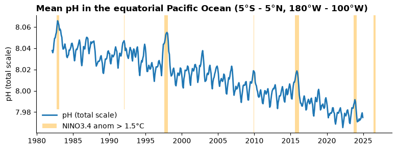
Visualisation
The ocean soda v2 dataset is in geozarr format. This means that the data is available at multiple resolutions and can be interactively visualised by any GeoZarr viewer by passing the dataset url. For example:
The viewer from the project team and the associated library (https://
github .com /lukegre /geozarr -pyramid -maker /tree /main) : https:// lukegre .github .io /geozarr -pyramid -maker /viewer/ Through open-layers: https://
sunnydean .github .io /ocean _cubes _vis / ?cube = https:// s3 .waw4 -1 .cloudferro .com /EarthCODE /OSCAssets /ocean -soda /OceanSODA _ETHZv2 .r2026 .GCB -fgco2 -1982 _2025 -pyramid .zarr & variable = sfco2 Through gridlook - https://
gridlook .pages .dev / #https:// s3 .waw4 -1 .cloudferro .com /EarthCODE /OSCAssets /ocean -soda /OceanSODA _ETHZv2 .r2026 .GCB -fgco2 -1982 _2025 -pyramid .zarr
See the visualisation section for more info.
- Gregor, Luke, & Gruber, Nicolas. (2020). OceanSODA-ETHZ: A global gridded dataset of the surface ocean carbonate system for seasonal to decadal studies of ocean acidification (v2025) (NCEI Accession 0220059). NOAA National Centers for Environmental Information. 10.25921/M5WX-JA34