The MEDICANES atlas contains observations from different satellites over medicane events in Mediterranean Sea. All data are available at Ifremer : https://
In particular, the climatology folder contains observations from various satellite products colocated with Mediterranean storms, from 1991 to 2020. The storms are numbered from 513 (example: track00000513) to 1716 (track00001716). Each storm folder contains subfolders, for each observation product that was colocated with the storm trajectory. For instance for storm folder track00001556, the SCATSAT1-L2-ICM subfolder contains wind speed and direction by Indian scatterometer SCATSAT-1. The different passes of this satellite colocated with this storm are stored in time ordered subfolders (<year/day in the year>, for instance track00001556/SCATSAT1-L2-ICM/2017/040/
All storm trajectories are stored in the file (in parquet format): https://
Collecting data from the Atlas
Let’s collect for instance an observation file from SCATSAT-1 scatterometer for the storm track00001556:
import urllib.request
urllib.request.urlretrieve('https://data-cersat.ifremer.fr/data/storms/medicanes/storm-atlas/climatology/track00001586/SCATSAT1-L2-ICM/2018/033/20180202182824_track00001586_SCATSAT1-L2-ICM.nc', "20180202182824_track00001586_SCATSAT1-L2-ICM.nc")
('20180202182824_track00001586_SCATSAT1-L2-ICM.nc',
<http.client.HTTPMessage at 0x7026502de490>)Read and display
The file downloaded above is in satellite projection (swath along the satellite track). We can display its content easily:
import matplotlib.pyplot as plt
import numpy as np
import cartopy.crs as ccrs
import cartopy.feature as cfeature
from cartopy.mpl.gridliner import LONGITUDE_FORMATTER, LATITUDE_FORMATTER
import xarray as xr
First open the file and display its content:
ds = xr.open_dataset('20180202182824_track00001586_SCATSAT1-L2-ICM.nc')
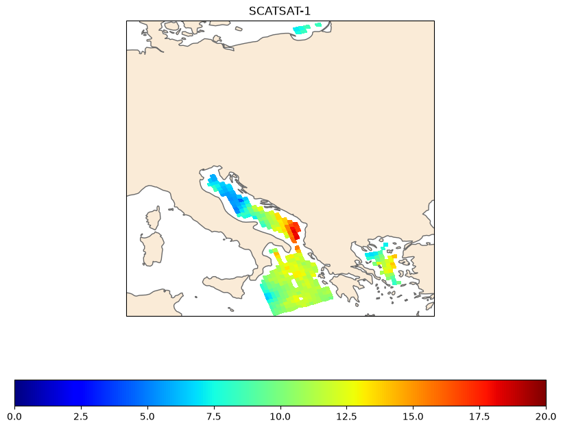
dsLet’s display the wind speed measured by the scatterometer:
# 1. Initialize the figure and map projection
fig = plt.figure(figsize=(10, 8))
ax = plt.axes(projection=ccrs.PlateCarree())

# 2. Add base map layers and features
ax.add_feature(cfeature.LAND.with_scale('50m'), facecolor='antiquewhite')
ax.add_feature(cfeature.COASTLINE, edgecolor='dimgray', linewidth=1)

# 3. Display the wind speed variable
# ignore the invalid lat/lon when plotting
valid = np.isfinite(ds.lon)
cax = ax.pcolormesh(ds.lon.where(valid, drop=True), ds.lat.where(valid, drop=True), ds.wind_speed.where(valid, drop=True), vmin=0,vmax=20, cmap='jet')

## Uncomment for gridlines
# 4. Configure gridlines and coordinate labels
# gl = ax.gridlines(crs=ccrs.PlateCarree(), draw_labels=True,
#                   linewidth=0.5, color='gray', alpha=0.5, linestyle='--')

# Disable labels on the top and right side for a cleaner layout
# gl.top_labels = False
# gl.right_labels = False

# Format labels to show degrees East/West and North/South
# gl.xformatter = LONGITUDE_FORMATTER
# gl.yformatter = LATITUDE_FORMATTER

plt.colorbar(cax, orientation='horizontal')

plt.title("SCATSAT-1")

# Save or display the map
plt.show()