Explore re-projected dataset in the Med cube
The careheat datababase has several datasets related to marine heatwaves (MHWs) and cold spells (MCSs).
careheat_mhw_2d.zarr - Events are identified for each pixel following the methodology of Hobday et al. (2016) with different preprocessing steps.
ssa_careheat_mhw_2d.zarr - Events are identified for each pixel following the methodology of Hobday et al. (2016) with different preprocessing steps.
careheat_mhw_metrics_2d.zarr - intensity, duration, heterogeneity and rate metrics for careheat_mhw_2d events.
ssa_careheat_mhw_metrics_2d.zarr - intensity, duration, heterogeneity and rate metrics for ssa_careheat_mhw_2d events.
careheat4d-med.zarr - 4d careheat events for the Mediterranian.
EO4SOCIETY Website: https://
eo4society .esa .int /projects /careheat/ Original Data Source: https://
zenodo .org /records /8154587 - not processed https:// data -cersat .ifremer .fr /data /marine -heat -wave /esa -careheat /cnr /v2/ https:// sextant .ifremer .fr /record /87a33c31 -5930 -4379 -8cfa -0b29ceee9756/ Reference: https://
opensciencedata .esa .int /projects /careheat /collection OSC entry: https://
opensciencedata .esa .int /projects /careheat /collection License: cc-by-4.0.
import xarray as xrfrom pystac_client import Client
catalog = Client.open("https://eoapi.workspace.earthcode.eox.at/stac/")
collection = catalog.search(collections=["careheat-database"]).item_collection()
items = {item.id: item for item in collection}
collection[item.assets["data"].href for item in collection]ds = xr.open_zarr(items["careheat-database-careheat_mhw_2d"].assets["data"].href)
dsimport matplotlib.pyplot as plt
import cartopy.crs as ccrs
import cartopy.feature as cfeature
from matplotlib.colors import BoundaryNorm
import numpy as np
date = "2020-06"
da = ds["category"].sel(time=np.datetime64(date), lon=slice(-6.062, 36.06), lat=slice(30.27, 45.98), drop=True)
# Categories present in the data
categories = [0, 1, 2, 3, 4]
# Discrete colormap
cmap = plt.get_cmap("viridis", len(categories))
# Put colour boundaries halfway between categories
bounds = [-0.5, 0.5, 1.5, 2.5, 3.5, 4.5]
norm = BoundaryNorm(bounds, cmap.N)
fig, ax = plt.subplots(
figsize=(12, 6),
subplot_kw={"projection": ccrs.PlateCarree()}
)
im = ax.pcolormesh(
da.lon,
da.lat,
da,
transform=ccrs.PlateCarree(),
cmap=cmap,
norm=norm,
shading="auto"
)
ax.coastlines()
ax.add_feature(cfeature.LAND, facecolor="lightgray")
labels = [
"No event",
"Moderate",
"Strong",
"Severe",
"Extreme"
]
cbar = fig.colorbar(
im,
ax=ax,
ticks=[0, 1, 2, 3, 4],
pad=0.03
)
cbar.ax.set_yticklabels(labels)
cbar.set_label("Marine Heatwaves category")
ax.set_title(f"Marine Heatwaves - {date}")
plt.show()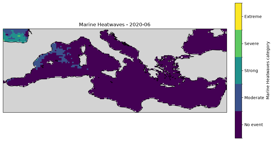
Metrics dataset
The “date_start” and “date_end” are another key part of the data.
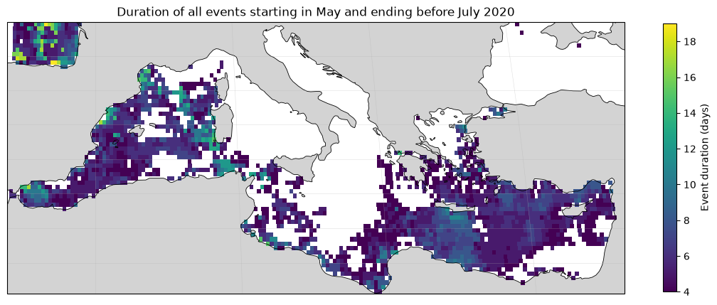
For example, one can compute the duration of a events at certain location by doing:
import pandas as pd

ds = xr.open_zarr(items["careheat-database-careheat_mhw_metrics_2d"].assets["data"].href)

# select all the date starts and date ends for the Med
dstart = ds["date_start"].sel(lon=slice(-6.062, 36.06), lat=slice(30.27, 45.98), drop=True)
dend = ds["date_end"].sel(lon=slice(-6.062, 36.06), lat=slice(30.27, 45.98), drop=True)dstart.isel(nevent=0).valuesarray([[ nan, nan, nan, ..., nan, nan,
nan],
[ nan, nan, nan, ..., nan, nan,
nan],
[ nan, nan, nan, ..., nan, nan,
nan],
...,
[19830710., 19830710., 19830713., ..., nan, 19820101.,
nan],
[19830710., 19830710., 19830710., ..., 19820101., 19801231.,
19801230.],
[19830710., 19830710., 19830710., ..., 19810209., 19801224.,
19801224.]], shape=(63, 168))keep = (dstart.values >= 20200501) & (dend.values < 20200700)
def parse_ymd(block):
    a = block.ravel()
    dates = pd.to_datetime(
        {
            "year": a // 10000,
            "month": (a // 100) % 100,
            "day": a % 100,
        },
        errors="coerce",
    )
    return dates.to_numpy(dtype="datetime64[ns]").reshape(block.shape)

def convert_dates(da):
    return xr.apply_ufunc(
        parse_ymd,
        da.where(keep),
        dask="parallelized",
        output_dtypes=[np.dtype("datetime64[ns]")],
    )

start = convert_dates(dstart)
end = convert_dates(dend)

duration_days = ((end - start) / np.timedelta64(1, "D")).rename(
    "duration_days"
)
duration_days.attrs = {"units": "days"}start.values[0]array([['NaT', 'NaT', 'NaT', ..., 'NaT', 'NaT', 'NaT'],
['NaT', 'NaT', 'NaT', ..., 'NaT', 'NaT', 'NaT'],
['NaT', 'NaT', 'NaT', ..., 'NaT', 'NaT', 'NaT'],
...,
['NaT', 'NaT', 'NaT', ..., 'NaT', 'NaT', 'NaT'],
['NaT', 'NaT', 'NaT', ..., 'NaT', 'NaT', 'NaT'],
['NaT', 'NaT', 'NaT', ..., 'NaT', 'NaT', 'NaT']],
shape=(63, 168), dtype='datetime64[ns]')# duration_days already contains only events starting in June
valid = duration_days.notnull()
# First valid event index at each grid cell
first = valid.argmax(dim="nevent").compute()
# Reduce to (lat, lon); mask cells with no matching event
monthly_duration = duration_days.isel(nevent=first).where(
valid.any(dim="nevent")
)import matplotlib.pyplot as plt
import cartopy.crs as ccrs
import cartopy.feature as cfeature
fig, ax = plt.subplots(
figsize=(14, 7),
subplot_kw={"projection": ccrs.Robinson()},
)
monthly_duration.plot.pcolormesh(
ax=ax,
x="lon",
y="lat",
transform=ccrs.PlateCarree(),
cmap="viridis",
cbar_kwargs={
"label": "Event duration (days)",
"shrink": 0.7,
},
)
ax.coastlines(linewidth=0.6)
ax.gridlines(linewidth=0.4, alpha=0.4)
ax.set_title("Duration of all events starting in May and ending before July 2020")
ax.add_feature(cfeature.LAND, facecolor="lightgray")
<cartopy.mpl.feature_artist.FeatureArtist at 0x14a04afd0>