Explore re-projected dataset in the Med cube
This dataset contains monthly Level-3 (L3) gridded maps (8 km resolution) of phytoplankton functional types (PFTs) and diffuse attenuation coefficients (Kd) for the period January 2019 to December 2021.
Original Data Source: https://
zenodo .org /records /17077474 Reference: https://
zenodo .org /records /17077474 OSC entry: https://
opensciencedata .esa .int /products /4dmed -2d -pft -kd /collection License: CC-BY-4.0
import xarray as xr
from pystac_client import Client

catalog = Client.open("https://eoapi.workspace.earthcode.eox.at/stac/")
item = next(catalog.search(collections=["4dmed-2d-pft-kd"], ids=["4dmed-2d-pft-kd-item-pft"]).items())
item
Loading...
item.assets["data"].hrefds = xr.open_zarr(item.assets["data"].href)
dsLoading...
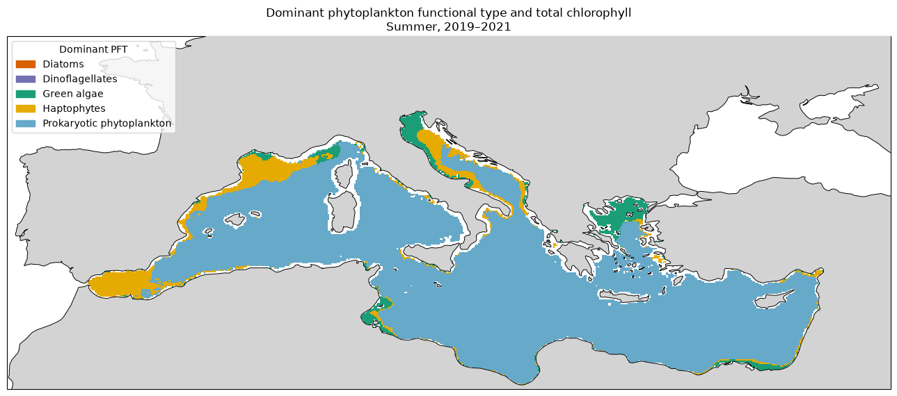
Plot the phytoplankton functional type contributing the most chlorophyll at each grid cell during the summer months
import numpy as np
import xarray as xr

pft_names = ["DIATO", "DINO", "GREEN", "HAPTO", "PROKA"]

pft = ds[pft_names].to_array(dim="pft")
summer = pft.sel(
    time=pft.time.dt.month.isin([6, 7, 8])
).mean("time")
total_chlorophyll is the combined chlorophyll concentration of the five groups. dominant_pft stores the index of the group with the highest concentration at each grid cell.
total_chlorophyll = summer.sum("pft", min_count=1)

dominant_pft = (
    summer.fillna(-np.inf)
    .argmax("pft")
    .where(total_chlorophyll.notnull())
)

total_chlorophyll = total_chlorophyll.compute()
dominant_pft = dominant_pft.compute()
import matplotlib.pyplot as plt
import matplotlib.patches as mpatches
from matplotlib.colors import ListedColormap, BoundaryNorm
import cartopy.crs as ccrs
import cartopy.feature as cfeature
pft_colours = [
"#d95f02", # Diatoms
"#7570b3", # Dinoflagellates
"#1b9e77", # Green algae
"#e6ab02", # Haptophytes
"#66a9c9", # Prokaryotic phytoplankton
]
pft_labels = [
"Diatoms",
"Dinoflagellates",
"Green algae",
"Haptophytes",
"Prokaryotic phytoplankton",
]
cmap = ListedColormap(pft_colours)
norm = BoundaryNorm(np.arange(-0.5, 5.5, 1), cmap.N)
projection = ccrs.PlateCarree()
fig = plt.figure(figsize=(13, 7))
ax = plt.axes(projection=projection)
ax.set_extent(
[
float(ds.lon.min()),
float(ds.lon.max()),
float(ds.lat.min()),
float(ds.lat.max()),
],
crs=projection,
)
ax.pcolormesh(
ds.lon,
ds.lat,
dominant_pft,
cmap=cmap,
norm=norm,
shading="auto",
transform=projection,
)
ax.add_feature(cfeature.LAND, facecolor="lightgrey", zorder=3)
ax.coastlines(resolution="50m", linewidth=0.7, zorder=4)
legend_handles = [
mpatches.Patch(color=colour, label=label)
for colour, label in zip(pft_colours, pft_labels)
]
ax.legend(
handles=legend_handles,
title="Dominant PFT",
loc="upper left",
frameon=True,
)
ax.set_title(
"Dominant phytoplankton functional type and total chlorophyll\n"
"Summer, 2019–2021"
)
plt.tight_layout()
plt.show()