Explore re-projected dataset in the Med cube
This dataset provides monthly information on Cumulative Hazard Indexs (CHIs) at the sea surface (3D, lat, lon, time) at global scale. The dataset is split into 3 zarr stores:
Global CHI1 and CHI3 indicies
Global CHI2 indicies
Global CHI4 indicies
EO4SOCIETY Website: https://
eo4society .esa .int /projects /mitho/ Original Data Source: https://
zenodo .org /records /17191460 Reference: https://
opensciencedata .esa .int /products /global -cumulative -hazard -indexes -chis /collection .json OSC entry: https://
opensciencedata .esa .int /products /global -cumulative -hazard -indexes -chis /collection .json License: CC-BY-4.0
This tutorial accesses the published Zarr stores over HTTPS and illustrates the multistressor construction of CHI1, global July 2022 conditions, and annual changes across the Mediterranean and four subbasins: Western Mediterranean, Adriatic, Ionian, and Levantine–Aegean. The monthly map shows July 2022; time series cover the full record.
The Mediterranean is used here as a regional example to illustrate basin-scale and subbasin-scale analyses. A global map provides context; basin analyses are examples, not a geographic restriction of the data.
Source: original NetCDF dataset on Zenodo · catalogue entry · MiTHo
| Index | Inputs / stressors | Available period | Levels |
|---|---|---|---|
| CHI1 | Sea surface temperature (SST): warm and cold extremes; hydrogen ion concentration (H+): acidification | Jan 1993–Dec 2022 | Surface |
| CHI2 | Temperature: warm and cold extremes; dissolved oxygen: deoxygenation; salinity: low and high extremes | Jan 2004–Nov 2022 | 2.5 dbar (level=0), 200 dbar (level=1) |
| CHI3 | SST, H+, sea surface salinity (SSS), sea surface density (SSD), wind speed: nine stressors in total | Jan 1993–Dec 2022 | Surface |
| CHI4 | SST: warm and cold extremes; fishing effort (FE): high values | Jan 2012–Dec 2020 | Surface |
The dataset is gridded on a 1° x 1° regular lat-lon grid.
Geographic coverage and valid-data masks differ between indices.
CHI3 combines both low and high extremes of SSS, SSD and wind in a single index.
For any given variable and threshold pair, low and high extremes are mutually exclusive
at the same place and time. Extremes of different variables can occur together.
1. Environment and required input files
The CHI stores use Zarr format 3.
Keep these files together:
mitho_access.ipynb
inputs/
    mediterranean_subbasin_masks_1deg.nc
The basin-mask NetCDF is a ready-to-use input file distributed with this notebook. The notebook reads it without modifying it; it does not create, resample or export a basin-mask file. No original high-resolution masks are needed. The input path can be changed in the settings below.
Figures, tables and run information are saved in notebook_artifacts/.
Access to the public CHI data requires internet. Cartopy may also download
Natural Earth coastline and land files on the first run.
# Libraries for arrays, remote data, tables and maps.
from pathlib import Path
import importlib.metadata as metadata
import json
import urllib.request
import numpy as np
import pandas as pd
import xarray as xr
import dask
import matplotlib.pyplot as plt
import matplotlib.colors as mcolors
from matplotlib.patches import Patch
import cartopy
import cartopy.crs as ccrs
import cartopy.feature as cfeature
from IPython.display import display
Create the output directory and display the package versions used for this run.
# Keep generated files together; do not modify the source data.
ARTIFACTS = Path("notebook_artifacts")
ARTIFACTS.mkdir(exist_ok=True)
cartopy.config["data_dir"] = ARTIFACTS / "cartopy_data"
packages = [
    "numpy",
    "xarray",
    "zarr",
    "fsspec",
    "aiohttp",
    "dask",
    "matplotlib",
    "cartopy",
]
versions = {name: metadata.version(name) for name in packages}
display(pd.Series(versions, name="Installed version").to_frame())
assert (
    int(versions["zarr"].split(".")[0]) >= 3
), "Install the supplied Zarr 3 environment."2. Locate and open the published data
The first store contains CHI1 and CHI3, using CH1_ and CH3_ prefixes.
The other stores contain CHI2 and CHI4. Fetching each store’s root metadata below
checks that all three URLs expose Zarr 3 groups, without loading their data arrays.
from pystac_client import Client

catalog = Client.open("https://eoapi.workspace.earthcode.eox.at/stac/")
collection = catalog.search(collections=["global-cumulative-hazard-indexes-chis"]).item_collection()
items = {item.id: item for item in collection}

# The three published datasets.
STORES = {
    "CHI1 / CHI3": items["global-cumulative-hazard-indexes-chis-mitho-ch13"],
    "CHI2": items["global-cumulative-hazard-indexes-chis-mitho-chi2_2004_2022"],
    "CHI4": items["global-cumulative-hazard-indexes-chis-mitho-chi4_2012_2020"],
}
collection[item.assets["data"].href for item in collection]Fetch the small root metadata from each store to check access. This does not download the full datasets.
# Read one metadata document per store.
store_checks = []
for label, source_item in STORES.items():
    with urllib.request.urlopen(source_item.assets["data"].href + "/zarr.json", timeout=60) as response:
        root = json.load(response)
    assert root["zarr_format"] == 3 and root["node_type"] == "group"
    store_checks.append(
        {"Indices": label, "Zarr format": root["zarr_format"], "Metadata": "accessible"}
    )
display(pd.DataFrame(store_checks))Open the CHI1/CHI3 store lazily: xarray reads metadata now and numerical chunks only when requested.
# Dask keeps data lazy until a later compute() call.
ds = xr.open_zarr(STORES["CHI1 / CHI3"].assets["data"].href, consolidated=True, chunks={})
ds3. What does CHI1 represent?
The original processing code constructs the unnormalized CHI1 as:
CHI1 = S_MHW + S_CS + S_PH
S_MHW is the marine-heatwave contribution, S_CS the cold-spell contribution,
and S_PH the acidification contribution. They are non-negative, dimensionless
stressor intensities derived from standardized anomalies at detected extremes.
They are not raw SST or pH measurements. For SST, the processing uses monthly
90th/10th percentile thresholds for warm/cold extremes, respectively.
The example uses the unnormalized, fixed-climatology variables. _mav identifies
the alternative based on a moving climatology, rather than simply a smoothed CHI
time series. _norm, _mean, _std, _Cat and _PI identify other derived products;
they are not interchangeable with the variables plotted here.
Higher CHI values indicate a larger sum of stressor contributions under this method; they are not calibrated probabilities of ecological damage. The baseline depends on the input product and must be considered when comparing different indices.
For CHI1, _norm divides the raw index by the global spatial maximum of each month.
The global context below uses raw CHI1, not this normalized variant.
# Names and example settings can be changed here.
VARIABLES = ["CH1_CHI1", "CH1_S_MHW", "CH1_S_CS", "CH1_S_PH"]
LABELS = [
    "CHI1 — cumulative index",
    "Marine heatwave contribution",
    "Cold-spell contribution",
    "Acidification contribution",
]
assert set(VARIABLES).issubset(ds.data_vars)
assert all(ds[v].dims == ("time", "latitude", "longitude") for v in VARIABLES)

DATE = "2022-07"
MASK_FILE = Path("inputs/mediterranean_subbasin_masks_1deg.nc")
LON_BOUNDS = (-6.062, 36.06)
LAT_BOUNDS = (30.27, 45.98)
A small helper keeps geographic slicing valid for either coordinate ordering.
# Reverse the slice if coordinates run from north to south.
def coordinate_slice(coord, bounds):
    # Support both ascending and descending latitude/longitude coordinates.
    return (
        slice(*bounds) if coord.values[0] < coord.values[-1] else slice(*bounds[::-1])
    )


DYNAMIC_VARIABLES = VARIABLES + ["CH1_CHI1_norm"]
Select only the variables and geographic rectangle needed for the regional example.
# Selection is still lazy; no numerical arrays are loaded yet.
subset = ds[DYNAMIC_VARIABLES].sel(
    longitude=coordinate_slice(ds.longitude, LON_BOUNDS),
    latitude=coordinate_slice(ds.latitude, LAT_BOUNDS),
)
assert subset.sizes["latitude"] > 0 and subset.sizes["longitude"] > 0
print("Native chunks:", {v: ds[v].encoding.get("chunks") for v in VARIABLES})
print("Subset dimensions:", dict(subset.sizes))

# Read only these five variables, with bounded concurrent chunk decompression.
# Native chunks are large: a small map/point may still require substantial I/O.
Native chunks: {'CH1_CHI1': (180, 180, 360), 'CH1_S_MHW': (180, 180, 360), 'CH1_S_CS': (180, 180, 360), 'CH1_S_PH': (180, 180, 360)}
Subset dimensions: {'time': 360, 'latitude': 16, 'longitude': 42}
Load the selected regional data once, then extract the July 2022 map.
# Limit concurrent decompression because the native chunks are large.
with dask.config.set(scheduler="threads", num_workers=2):
    regional = subset.compute()

selected_month = regional.sel(time=DATE)
assert selected_month.sizes["time"] == 1, "Expected one monthly sample."
snapshot = selected_month.isel(time=0, drop=True)
4. Read the supplied Mediterranean basin-mask file
inputs/mediterranean_subbasin_masks_1deg.nc already contains masks on the
same 1° grid as the CHI data, with these variables:
| Variable in the file | Region |
|---|---|
Mediterranean | Whole Mediterranean |
Western_Mediterranean | Western Mediterranean |
Adriatic_Sea | Adriatic |
Ionian_Sea | Ionian |
Levantine_Aegean_Sea | Levantine–Aegean |
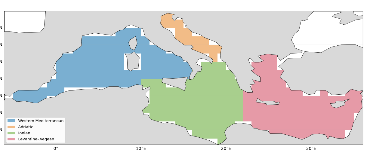
Values are 1 inside each supplied mask and 0 outside it. The code selects the matching grid coordinates directly: it performs no interpolation or regridding.
For the analysis, cells without CHI1 data are excluded. This is a data-availability filter, not a change to the supplied basin boundaries. Fixed temporal coverage is applied later when computing the means. The following map visualizes the regions read from the file on the CHI marine-data footprint.
# Read the ready-made input file and select matching coordinates exactly.
if not MASK_FILE.is_file():
    raise FileNotFoundError(f"Place the supplied basin-mask NetCDF at {MASK_FILE}")

with xr.open_dataset(MASK_FILE, engine="netcdf4") as source:
    mask_data = source.load().sel(
        latitude=regional.latitude, longitude=regional.longitude
    )
REGIONS = {
    "Western Mediterranean": "Western_Mediterranean",
    "Adriatic": "Adriatic_Sea",
    "Ionian": "Ionian_Sea",
    "Levantine–Aegean": "Levantine_Aegean_Sea",
}
COLOURS = {
    "Mediterranean": "#202020",
    "Western Mediterranean": "#3888bc",
    "Adriatic": "#d88b3c",
    "Ionian": "#54a44b",
    "Levantine–Aegean": "#ca5b76",
}
raw_submasks = {name: mask_data[key].astype(bool) for name, key in REGIONS.items()}
raw_med_mask = mask_data["Mediterranean"].astype(bool)
Exclude cells without CHI1 observations, while keeping the supplied region assignments.
# Filter data availability; do not modify or write the supplied mask file.
marine_footprint = np.isfinite(regional.CH1_CHI1).any("time")
submasks = {name: mask & marine_footprint for name, mask in raw_submasks.items()}
membership = xr.concat(list(submasks.values()), dim="basin").sum("basin")
assert not bool(
    (membership > 1).any()
), "Overlapping marine cells require a mask review."
med_mask = raw_med_mask & marine_footprint
basin_masks = {"Mediterranean": med_mask, **submasks}
snapshot = snapshot.where(med_mask)

# Record the input path and run settings, not a newly generated mask.
validation = {
    "source": STORES["CHI1 / CHI3"].assets["data"].href,
    "date": DATE,
    "versions": versions,
    "mask_input_file": MASK_FILE.as_posix(),
    "mask_alignment": "Exact coordinate selection from the supplied 1-degree NetCDF; no resampling",
}
Visualize the regions read from the input file. Colours are display labels only.
# Assign one plotting colour to each subbasin.
class_map = xr.full_like(med_mask, np.nan, dtype=float)
for i, mask in enumerate(submasks.values()):
    class_map = xr.where(mask, i, class_map)
fig, ax = plt.subplots(
    figsize=(12, 5), subplot_kw={"projection": ccrs.PlateCarree()}, layout="constrained"
)
palette = ["#7aafd1", "#f2bc87", "#a8cf8d", "#e69aa7"]
ax.pcolormesh(
    class_map.longitude,
    class_map.latitude,
    class_map,
    shading="auto",
    transform=ccrs.PlateCarree(),
    cmap=mcolors.ListedColormap(palette),
    vmin=-0.5,
    vmax=3.5,
)
ax.add_feature(cfeature.LAND.with_scale("110m"), facecolor="0.85", zorder=3)
ax.coastlines(resolution="110m", linewidth=0.6, zorder=4)
ax.set_extent([*LON_BOUNDS, *LAT_BOUNDS], crs=ccrs.PlateCarree())
gl = ax.gridlines(draw_labels=True, linewidth=0.3, alpha=0.4)
gl.top_labels = False
gl.right_labels = False
ax.legend(
    handles=[
        Patch(facecolor=colour, label=name) for name, colour in zip(REGIONS, palette)
    ],
    loc="lower left",
    fontsize=9,
    framealpha=0.95,
)
ax.set_title("Mediterranean subbasins — supplied masks on the 1° CHI grid")
fig.savefig(
    ARTIFACTS / "mediterranean_subbasin_masks.png", dpi=160, bbox_inches="tight"
)
plt.show()
/Users/dean/code/ocean_hackathon/.pixi/envs/default/lib/python3.13/site-packages/cartopy/io/__init__.py:242: DownloadWarning: Downloading: https://naturalearth.s3.amazonaws.com/110m_physical/ne_110m_land.zip
warnings.warn(f'Downloading: {url}', DownloadWarning)
/Users/dean/code/ocean_hackathon/.pixi/envs/default/lib/python3.13/site-packages/cartopy/io/__init__.py:242: DownloadWarning: Downloading: https://naturalearth.s3.amazonaws.com/110m_physical/ne_110m_coastline.zip
  warnings.warn(f'Downloading: {url}', DownloadWarning)
5. Global context: raw CHI1 in July 2022
Use a monthly map of the unnormalized CHI1, rather than a full-period count. This retains the spatial contrast between places with no detected stressors and places with larger cumulative intensities in the selected month. The colour scale covers the actual minimum of zero to the maximum in this map; values are not clipped to a percentile. White marine cells have no data.
The blue rectangle locates the Mediterranean example. The map is a snapshot, not a temporal trend or a calibrated ecological-risk map.
# Read a single monthly field on the full global grid.
global_month = ds["CH1_CHI1"].sel(time=DATE)
assert global_month.sizes["time"] == 1
with dask.config.set(scheduler="threads", num_workers=2):
    global_snapshot = global_month.isel(time=0, drop=True).compute()

global_colour_max = float(global_snapshot.max(skipna=True))
print(f"Raw global CHI1 in {DATE}: 0 to {global_colour_max:.3f}")
Raw global CHI1 in 2022-07: 0 to 7.304
Draw the global map using its own colour scale, in raw dimensionless CHI1 units.
fig = plt.figure(figsize=(13, 5.3), layout="constrained")
ax = fig.add_subplot(111, projection=ccrs.Robinson())
im = ax.pcolormesh(
    global_snapshot.longitude,
    global_snapshot.latitude,
    global_snapshot,
    transform=ccrs.PlateCarree(),
    shading="auto",
    cmap="viridis",
    vmin=0,
    vmax=global_colour_max,
)
ax.set_global()
ax.add_feature(cfeature.LAND.with_scale("110m"), facecolor="0.85", zorder=3)
ax.coastlines(resolution="110m", linewidth=0.4, zorder=4)

# Outline the regional selection without implying a restriction of the dataset.
ax.plot(
    [LON_BOUNDS[0], LON_BOUNDS[1], LON_BOUNDS[1], LON_BOUNDS[0], LON_BOUNDS[0]],
    [LAT_BOUNDS[0], LAT_BOUNDS[0], LAT_BOUNDS[1], LAT_BOUNDS[1], LAT_BOUNDS[0]],
    transform=ccrs.PlateCarree(),
    color="#2499df",
    linewidth=1.3,
    zorder=5,
)
fig.colorbar(
    im,
    ax=ax,
    orientation="horizontal",
    shrink=0.7,
    pad=0.04,
    label="Raw CHI1 (dimensionless)",
)
ax.set_title(f"Global CHI1 — {DATE}; Mediterranean example outlined in blue")
fig.savefig(ARTIFACTS / "chi1_global_2022-07.png", dpi=160, bbox_inches="tight")
plt.show()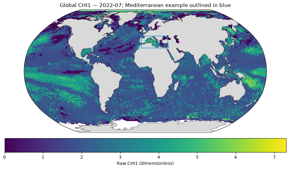
6. CHI1 and its three contributions in July 2022
All panels use the same linear colour scale so the magnitude of the contributions can be compared directly. Land is grey; missing marine values are left blank. Only Mediterranean grid-cell centres selected by the geographic mask below are plotted. The basin time series below use these four subbasins and their union.
# A common scale allows direct magnitude comparisons between the four panels.
values = snapshot[VARIABLES].to_array().values
finite_values = values[np.isfinite(values)]
assert finite_values.size > 0
vmax = float(finite_values.max())
norm = mcolors.Normalize(vmin=0, vmax=max(vmax, 1e-12))
cmap = plt.colormaps["viridis"].copy()
cmap.set_bad("white")
Draw the cumulative index and its components with the same colour limits.
# Use the same date, grid and geographic mask in every panel.
fig, axes = plt.subplots(
    2,
    2,
    figsize=(13, 6),
    subplot_kw={"projection": ccrs.PlateCarree()},
    layout="constrained",
)
for ax, variable, label in zip(axes.flat, VARIABLES, LABELS):
    field = snapshot[variable]
    mesh = ax.pcolormesh(
        field.longitude,
        field.latitude,
        field,
        transform=ccrs.PlateCarree(),
        shading="auto",
        cmap=cmap,
        norm=norm,
    )
    ax.set_extent([*LON_BOUNDS, *LAT_BOUNDS], crs=ccrs.PlateCarree())
    ax.add_feature(cfeature.LAND.with_scale("110m"), facecolor="0.85", zorder=3)
    ax.coastlines(resolution="110m", linewidth=0.6, zorder=4)
    gl = ax.gridlines(draw_labels=True, linewidth=0.3, alpha=0.4)
    gl.top_labels = False
    gl.right_labels = False
    ax.set_title(label, fontsize=11)
fig.colorbar(
    mesh,
    ax=list(axes.flat),
    label="Dimensionless index / stressor contribution",
    shrink=0.85,
    pad=0.03,
)
fig.suptitle(f"MiTHo CHI1 and component stressors — {DATE}", fontsize=15)
fig.savefig(ARTIFACTS / "chi1_components_2022-07.png", dpi=160, bbox_inches="tight")
plt.show()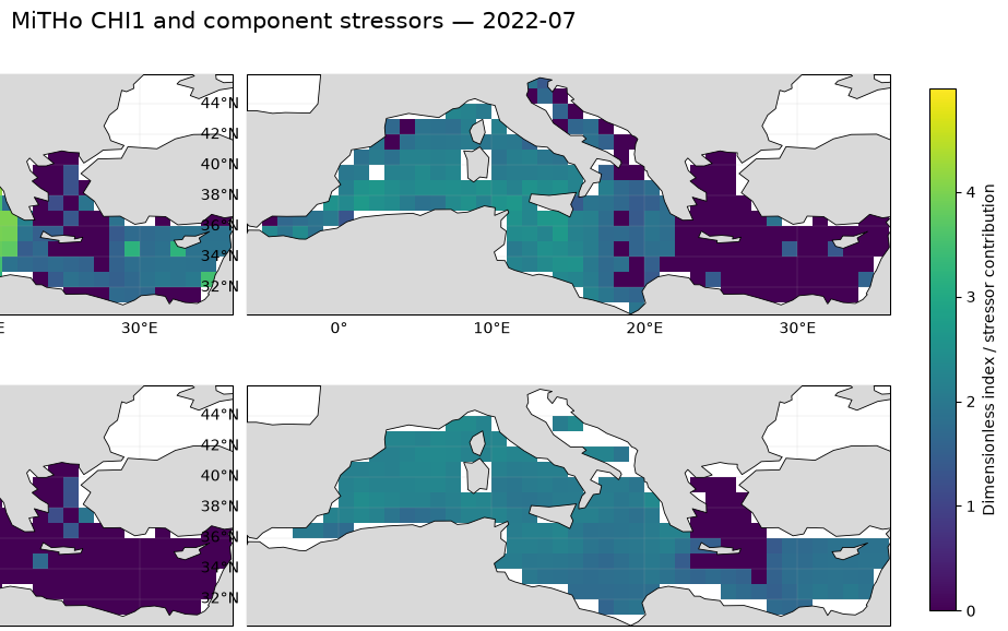
7. Monthly time series for the Mediterranean and four subbasins
Use the same spatial sample in every month: only cells with finite CHI1,
normalized CHI1 and all three contributions throughout 1993–2022 are retained.
Weights are proportional to cos(latitude). Missing areas are not filled or
extrapolated. The coverage table reports how much of each CHI marine footprint
is retained. Subbasin means use the supplied boundaries, not rectangular selections.
Each panel shows basin-mean CHI1 and its three contributions, on a common y scale. The dashed line marks July 2022. All 360 monthly samples are shown without smoothing.
# Keep the same complete-data cells throughout the record.
all_complete = (
    np.isfinite(regional[DYNAMIC_VARIABLES].to_array("variable"))
    .all("variable")
    .all("time")
)
lat_weights = np.cos(np.deg2rad(regional.latitude)).broadcast_like(med_mask)
coverage_rows, basin_weights, basin_monthly_fields = [], {}, {}
monthly_frames = []
Compute one area-weighted monthly series per basin for each variable.
# Cosine latitude weights account for cell-area differences on the regular grid.
for name, mask in basin_masks.items():
    retained = mask & all_complete
    assert int(retained.sum()) > 0, f"No complete cells in {name}"
    w = lat_weights.where(retained, 0)
    basin_weights[name] = w
    fields = regional[VARIABLES].weighted(w).mean(("latitude", "longitude"))
    basin_monthly_fields[name] = fields
    coverage_rows.append(
        {
            "Basin": name,
            "CHI marine grid cells": int(mask.sum()),
            "Retained complete cells": int(retained.sum()),
            "Retained area fraction (%)": float(
                100 * w.sum() / lat_weights.where(mask, 0).sum()
            ),
        }
    )
    frame = fields.to_dataframe()[VARIABLES].reset_index()
    frame.insert(0, "Basin", name)
    monthly_frames.append(frame)
Inspect the retained coverage before interpreting the basin means.
# Export the series and coverage so the numerical results can be inspected.
coverage_table = pd.DataFrame(coverage_rows)
display(coverage_table.round(2))
coverage_table.to_csv(ARTIFACTS / "basin_coverage.csv", index=False)
pd.concat(monthly_frames, ignore_index=True).to_csv(
    ARTIFACTS / "basin_monthly_series.csv", index=False
)Plot each basin separately so that the individual contributions remain readable.
# All panels share one vertical scale; the dashed line marks July 2022.
fig, axes = plt.subplots(
    5, 1, figsize=(13, 12), sharex=True, sharey=True, layout="constrained"
)
curve_labels = ["CHI1", "Marine heatwaves", "Cold spells", "Acidification"]
curve_colours = ["#202020", "#d95f02", "#2474b5", "#7b3294"]
for ax, (name, fields) in zip(axes, basin_monthly_fields.items()):
    for variable, label, colour in zip(VARIABLES, curve_labels, curve_colours):
        ax.plot(
            fields.time,
            fields[variable],
            label=label,
            color=colour,
            lw=1.3 if variable == "CH1_CHI1" else 0.85,
        )
    ax.axvline(np.datetime64("2022-07-01"), color="0.45", ls="--", lw=0.9)
    coverage = next(row for row in coverage_rows if row["Basin"] == name)
    ax.set_title(
        f"{name} — retained area {coverage['Retained area fraction (%)']:.1f}% "
        f"({coverage['Retained complete cells']}/{coverage['CHI marine grid cells']} marine cells)",
        loc="left",
        color=COLOURS[name],
        fontsize=10,
    )
    ax.set_ylabel("Mean CHI1 / contribution")
    ax.grid(alpha=0.2)
global_ymax = max(
    float(fields.to_array().max()) for fields in basin_monthly_fields.values()
)
axes[0].set_ylim(0, global_ymax * 1.05)
axes[0].legend(loc="upper left", ncol=4, fontsize=9)
axes[-1].set_xlim(regional.time.values[0], regional.time.values[-1])
axes[-1].set_xlabel("Time")
fig.suptitle(
    "Monthly CHI1 and stressors — fixed basin masks, area weighting", fontsize=14
)
fig.savefig(
    ARTIFACTS / "chi1_mediterranean_subbasin_monthly_series.png",
    dpi=160,
    bbox_inches="tight",
)
plt.show()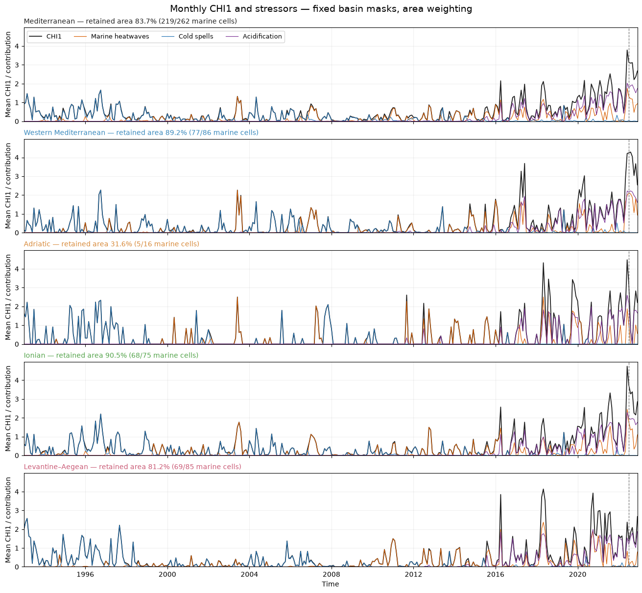
8. Basin-wide annual evolution: are recent extremes stronger or more frequent?
Keep the same spatial sample in every month: retain basin grid cells with finite
CHI1, normalized CHI1 and all three contributions for all 360 months.
Use weights proportional to cos(latitude) for the equal-angle grid. The coverage
table reports the retained fraction of each geographic mask; results describe those
observed cells, not an extrapolation to missing parts of the basin.
Three metrics separate different aspects:
Mean CHI1: mean over retained basin cells and all months of each year, including zeros.
Affected area: annual mean of the monthly area fraction satisfying
CHI1_norm > 1e-4.Intensity when active: annual weighted mean raw CHI1 across the active cell-months only.
The last metric helps separate magnitude from occurrence. An increase in mean CHI1 alone does not establish that individual extremes became stronger. These are descriptive comparisons under a fixed-climatology index, not a trend-significance or attribution test.
# Aggregate the monthly data by calendar year; active intensity excludes inactive cell-months.
annual_rows, decade_rows = [], []
basin_monthly = {}
for name, mask in basin_masks.items():
    w = basin_weights[name]
    retained = w > 0
    total_w = w.sum()
    field = regional.CH1_CHI1.where(retained)
    active = (regional.CH1_CHI1_norm > 1e-4) & retained
    monthly_mean = field.weighted(w).mean(("latitude", "longitude"))
    active_weight = w.where(active, 0).sum(("latitude", "longitude"))
    active_sum = (field.where(active, 0) * w).sum(("latitude", "longitude"))
    monthly_fraction = 100 * active_weight / total_w
    annual_mean = monthly_mean.resample(time="YS").mean()
    annual_area = monthly_fraction.resample(time="YS").mean()
    annual_intensity = (
        active_sum.resample(time="YS").sum() / active_weight.resample(time="YS").sum()
    )
    basin_monthly[name] = {
        "mean": monthly_mean,
        "area": monthly_fraction,
        "active_sum": active_sum,
        "active_weight": active_weight,
    }
    for i, time in enumerate(annual_mean.time.values):
        annual_rows.append(
            {
                "Basin": name,
                "Year": pd.Timestamp(time).year,
                "Mean CHI1": float(annual_mean[i]),
                "Affected area (%)": float(annual_area[i]),
                "Intensity when active": float(annual_intensity[i]),
            }
        )
    for label, start, end in [
        ("1993–2002", "1993", "2002"),
        ("2013–2022", "2013", "2022"),
    ]:
        s = slice(start, end)
        decade_rows.append(
            {
                "Basin": name,
                "Period": label,
                "Mean CHI1": float(monthly_mean.sel(time=s).mean()),
                "Affected area (%)": float(monthly_fraction.sel(time=s).mean()),
                "Intensity when active": float(
                    active_sum.sel(time=s).sum() / active_weight.sel(time=s).sum()
                ),
            }
        )
Display and save the annual and first/last-decade summaries.
# The coverage table remains the reference for interpreting every mean.
annual_table = pd.DataFrame(annual_rows)
decade_table = pd.DataFrame(decade_rows)
display(coverage_table.round(2))
display(decade_table.round(3))
coverage_table.to_csv(ARTIFACTS / "basin_coverage.csv", index=False)
annual_table.to_csv(ARTIFACTS / "basin_annual_metrics.csv", index=False)
decade_table.to_csv(ARTIFACTS / "basin_decade_comparison.csv", index=False)Compare three complementary metrics; a higher mean index can reflect frequency as well as intensity.
# Use separate axes for index magnitude, affected fraction and conditional intensity.
fig, axes = plt.subplots(3, 1, figsize=(12, 9), sharex=True, layout="constrained")
metric_labels = [
    ("Mean CHI1", "Basin mean CHI1"),
    ("Affected area (%)", "Mean monthly affected area (%)"),
    ("Intensity when active", "Raw CHI1 in active cell-months"),
]
for ax, (metric, label) in zip(axes, metric_labels):
    for name, colour in COLOURS.items():
        table = annual_table[annual_table.Basin == name]
        ax.plot(
            table.Year,
            table[metric],
            label=name,
            color=colour,
            lw=1.8,
            marker="o",
            ms=3,
        )
    ax.axvspan(1993, 2002, color="0.5", alpha=0.08)
    ax.axvspan(2013, 2022, color="0.5", alpha=0.08)
    ax.set_ylabel(label)
    ax.set_ylim(bottom=0)
    ax.grid(alpha=0.2)
    ax.legend(loc="upper left", ncol=3, fontsize=8)
axes[-1].set_xlabel("Year")
axes[-1].set_xlim(1993, 2022)
fractions = {row["Basin"]: row["Retained area fraction (%)"] for row in coverage_rows}
fig.suptitle(
    "CHI1 annual evolution — Mediterranean and four subbasins\nFixed complete-data masks and area weighting",
    fontsize=13,
)
fig.savefig(ARTIFACTS / "chi1_basin_annual_metrics.png", dpi=160, bbox_inches="tight")
plt.show()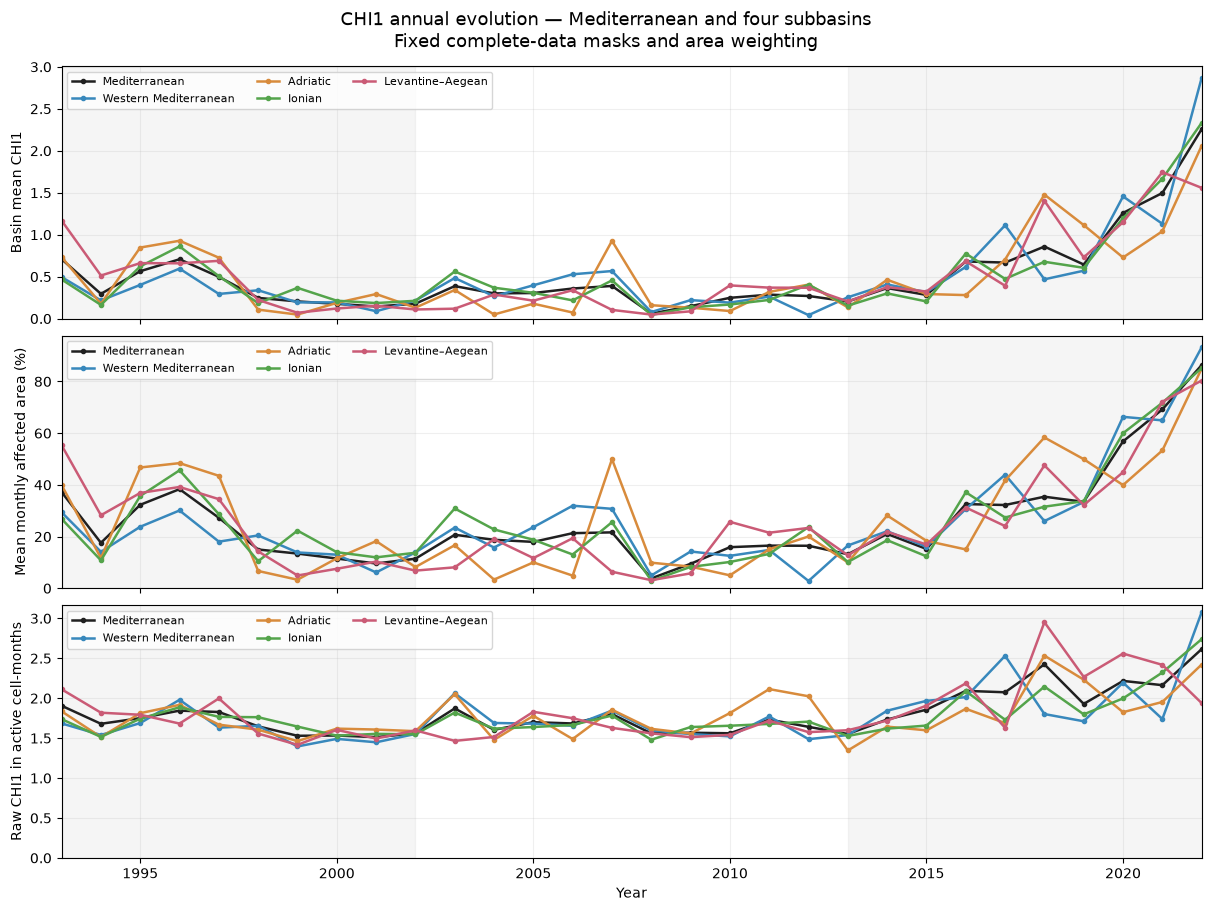
9. Spatial comparison of the first and last decades
Compare raw mean CHI1 in 1993–2002 and 2013–2022 using the same complete-data Mediterranean cells. Positive differences indicate larger mean cumulative intensity, which can reflect changes in both occurrence and magnitude. No significance test is applied.
# Retain the same complete-data cells in both decades.
retained_med = med_mask & all_complete
early = (
    regional.CH1_CHI1.sel(time=slice("1993", "2002")).mean("time").where(retained_med)
)
late = (
    regional.CH1_CHI1.sel(time=slice("2013", "2022")).mean("time").where(retained_med)
)
change = late - early
common_max = max(float(early.max()), float(late.max()), 1e-12)
change_max = max(float(abs(change).max()), 1e-12)
Compare the two decade means on a shared scale and map their difference separately.
# The difference uses a symmetric diverging colour scale centred on zero.
fig, axes = plt.subplots(
    1,
    3,
    figsize=(15, 4.2),
    subplot_kw={"projection": ccrs.PlateCarree()},
    layout="constrained",
)
for i, (ax, field, title) in enumerate(
    zip(
        axes,
        [early, late, change],
        [
            "Mean CHI1: 1993–2002",
            "Mean CHI1: 2013–2022",
            "Difference: last − first decade",
        ],
    )
):
    kwargs = (
        {"cmap": "viridis", "vmin": 0, "vmax": common_max}
        if i < 2
        else {"cmap": "RdBu_r", "vmin": -change_max, "vmax": change_max}
    )
    im = ax.pcolormesh(
        field.longitude,
        field.latitude,
        field,
        shading="auto",
        transform=ccrs.PlateCarree(),
        **kwargs
    )
    ax.set_extent([*LON_BOUNDS, *LAT_BOUNDS], crs=ccrs.PlateCarree())
    ax.add_feature(cfeature.LAND.with_scale("110m"), facecolor="0.85", zorder=3)
    ax.coastlines(resolution="110m", linewidth=0.5)
    ax.set_title(title, fontsize=10)
    fig.colorbar(
        im,
        ax=ax,
        orientation="horizontal",
        pad=0.06,
        shrink=0.9,
        label="Raw CHI1 (dimensionless)",
    )
fig.savefig(
    ARTIFACTS / "chi1_mediterranean_decade_change.png", dpi=160, bbox_inches="tight"
)
plt.show()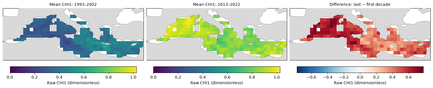
10. Mediterranean Persistency and Category maps
Use the stored products, and first verify them against the monthly normalized data. All maps cover the full 1993–2022 period:
Persistency: number of months with
CHI1_norm > 1e-4.Low Category: number of months with
0 < CHI1_norm <= 0.33.Medium Category: number of months with
0.33 < CHI1_norm <= 0.66.High Category: number of months with
0.66 < CHI1_norm <= 1.001.
The 1.001 upper bound is the numerical margin used in the source code; the nominal
normalized upper limit is 1. Category is relative to each month’s global spatial maximum,
not an absolute hazard threshold. Categories partition positive normalized values;
their total can differ from PI because PI excludes values at or below 1e-4.
These full-period counts locate repeated occurrence but do not themselves show whether events increased towards the end of the record. Use the annual metrics above for that question. Maps below retain the same complete-data Mediterranean mask. Each panel has its own colour scale in months, to make the rarer high category visible; compare the colourbar values, not colours alone, between panels.
# Load the supplied full-period count maps only when they are needed.
STATIC_VARIABLES = ["CH1_CHI1_PI", "CH1_CHI1_Cat"]
with dask.config.set(scheduler="threads", num_workers=2):
    static_region = (
        ds[STATIC_VARIABLES]
        .sel(latitude=regional.latitude, longitude=regional.longitude)
        .compute()
    )
Check that the supplied counts agree with the monthly normalized index.
# Count months, not consecutive duration; preserve the original category thresholds.
norm_series = regional.CH1_CHI1_norm
computed_pi = (norm_series > 1e-4).sum("time")
pi = static_region.CH1_CHI1_PI
np.testing.assert_allclose(
    pi.values[retained_med.values], computed_pi.values[retained_med.values]
)
category = static_region.CH1_CHI1_Cat
assert category.sizes["intensity_class"] == 3
category_ranges = [(0, 0.33), (0.33, 0.66), (0.66, 1.001)]
for i, (lower, upper) in enumerate(category_ranges):
    recomputed = ((norm_series > lower) & (norm_series <= upper)).sum("time")
    stored = category.isel(intensity_class=i)
    np.testing.assert_allclose(
        stored.values[retained_med.values], recomputed.values[retained_med.values]
    )
print(
    "Stored PI and all three Category counts match monthly data on the retained Mediterranean mask."
)
Stored PI and all three Category counts match monthly data on the retained Mediterranean mask.
Draw PI and the three categories, each with its own explicitly labelled count scale.
# Different panels have different count ranges, so compare their colourbar values.
fig, axes = plt.subplots(
    2,
    2,
    figsize=(13, 7),
    subplot_kw={"projection": ccrs.PlateCarree()},
    layout="constrained",
)
fields = [pi] + [category.isel(intensity_class=i) for i in range(3)]
titles = [
    "Persistency: normalized CHI1 > 10⁻⁴",
    "Low Category: (0, 0.33]",
    "Medium Category: (0.33, 0.66]",
    "High Category: (0.66, 1.001]",
]
for ax, field, title in zip(axes.flat, fields, titles):
    field = field.where(retained_med)
    im = ax.pcolormesh(
        field.longitude,
        field.latitude,
        field,
        transform=ccrs.PlateCarree(),
        shading="auto",
        cmap="YlOrRd",
        vmin=0,
        vmax=max(float(field.max()), 1),
    )
    ax.set_extent([*LON_BOUNDS, *LAT_BOUNDS], crs=ccrs.PlateCarree())
    ax.add_feature(cfeature.LAND.with_scale("110m"), facecolor="0.85", zorder=3)
    ax.coastlines(resolution="110m", linewidth=0.5)
    for basin_mask in submasks.values():
        ax.contour(
            basin_mask.longitude,
            basin_mask.latitude,
            basin_mask.astype(float),
            levels=[0.5],
            colors=["0.35"],
            linewidths=0.5,
            transform=ccrs.PlateCarree(),
            zorder=5,
        )
    ax.set_title(title, fontsize=10)
    cb = fig.colorbar(
        im,
        ax=ax,
        orientation="horizontal",
        pad=0.05,
        shrink=0.9,
        label="Number of months (panel-specific scale)",
    )
    cb.locator = plt.MaxNLocator(nbins=5, integer=True)
    cb.update_ticks()
fig.suptitle(
    "Mediterranean CHI1 Persistency and Category, 1993–2022\nSupplied subbasin boundaries in grey",
    fontsize=14,
)
fig.savefig(
    ARTIFACTS / "chi1_mediterranean_persistency_categories.png",
    dpi=160,
    bbox_inches="tight",
)
plt.show()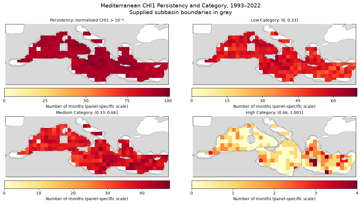
Save the run settings and close the remote dataset.
# Only derived outputs are written; source archives remain unchanged.
validation.update(
    {
        "basin_masks": list(basin_masks),
        "coverage": coverage_rows,
        "pi_and_category_counts_verified": True,
        "normalization": "raw CHI1 divided by its monthly global spatial maximum",
    }
)
(ARTIFACTS / "validation.json").write_text(
    json.dumps(validation, indent=2), encoding="utf-8"
)
ds.close()