Explore re-projected dataset in the Med cube
The gridded Sea Level Anomalies (SLA) presented here result from the application of the 4DVARNET algorithm, as described by Fablet et al., 2021. Here, the resolution of the dynamical model used for the learning/training (eNATL60-BLB02) is here downgraded to 1/8°. The algorithm takes as input Level-3 altimeter data distributed by the Copernicus Marine Service (European Union-Copernicus Marine Service (2021)). This product provides additional variables such as Absolute Dynamic Topography and geostrophic currents (both absolute values and anomalies) at a resolution of 1/24° over the Mediterranean Sea and for the period from 2016 to 2022. It is intended for delayed-time applications.
Original Data Source: https://
zenodo .org /records /10908416 Reference: Sammartino et al. (2022)
OSC entry: https://
opensciencedata .esa .int /products /4dmed -2d -alt -varnet -8 /collection License: CC-BY-4.0
import xarray as xr
import numpy as np
from pystac_client import Client

catalog = Client.open("https://eoapi.workspace.earthcode.eox.at/stac/")
item = next(catalog.search(collections=["4dmed-2d-alt-varnet-8"]).items())
itemitem.assets["data"].hrefds = xr.open_zarr(item.assets["data"].href)
dssnapshot = ds.sel(time="2016-05-22")
snapshotsla_limit = float(np.nanpercentile(np.abs(snapshot.sla), 98))import matplotlib.pyplot as plt
import matplotlib.lines as mlines
import cartopy.crs as ccrs
import cartopy.feature as cfeature
fig = plt.figure(figsize=(15, 8))
ax = plt.axes(projection=ccrs.PlateCarree())
ax.set_extent([
float(snapshot.longitude.min()),
float(snapshot.longitude.max()),
float(snapshot.latitude.min()),
float(snapshot.latitude.max())
], crs=ccrs.PlateCarree())
# Plot SLA with limits centred on zero so positive and negative anomalies are comparable
sla_plot = ax.pcolormesh(
snapshot.longitude,
snapshot.latitude,
snapshot.sla,
cmap="RdBu_r",
vmin=-sla_limit,
vmax=sla_limit,
shading="auto",
transform=ccrs.PlateCarree()
)
# Add coastlines and land to provide geographic context
ax.add_feature(cfeature.LAND, facecolor="0.88", zorder=3)
ax.coastlines(resolution="50m", linewidth=0.8, zorder=4)
ax.add_feature(cfeature.BORDERS, linewidth=0.4, zorder=4)
# Explain the SLA colours and vorticity contour meanings
colorbar = plt.colorbar(
sla_plot,
ax=ax,
orientation="horizontal",
pad=0.07,
fraction=0.05
)
colorbar.set_label("Sea-level anomaly (m)")
ax.set_title(
"Sea level anomalies - 22 May 2016"
)
plt.tight_layout()
plt.show()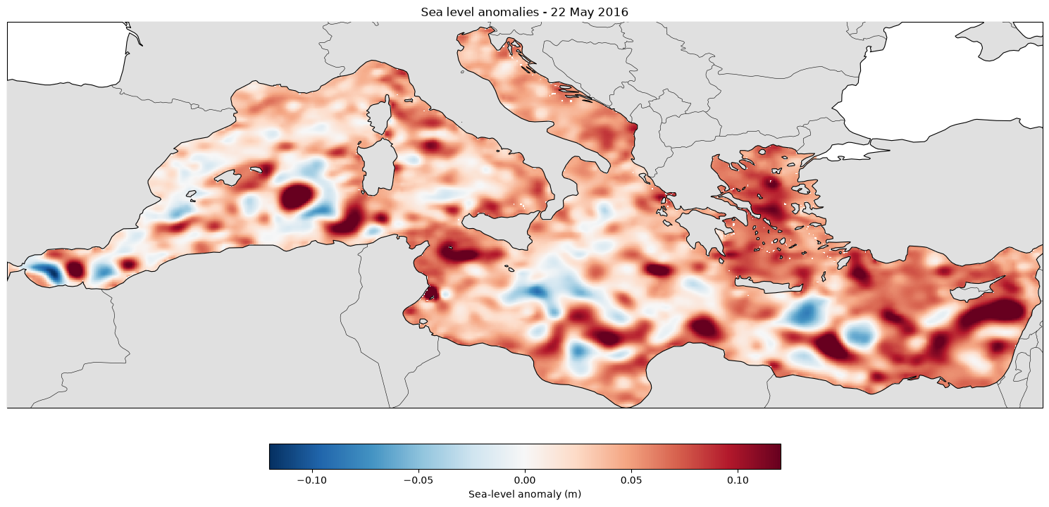
- European Union-Copernicus Marine Service. (2021). EUROPEAN SEAS ALONG-TRACK L3 SEA SURFACE HEIGHTS REPROCESSED (1993-ONGOING) TAILORED FOR DATA ASSIMILATION. Mercator Ocean International. 10.48670/MOI-00139
- Sammartino, M., Aronica, S., Santoleri, R., & Buongiorno Nardelli, B. (2022). Retrieving Mediterranean Sea Surface Salinity Distribution and Interannual Trends from Multi-Sensor Satellite and In Situ Data. Remote Sensing, 14(10), 2502. 10.3390/rs14102502