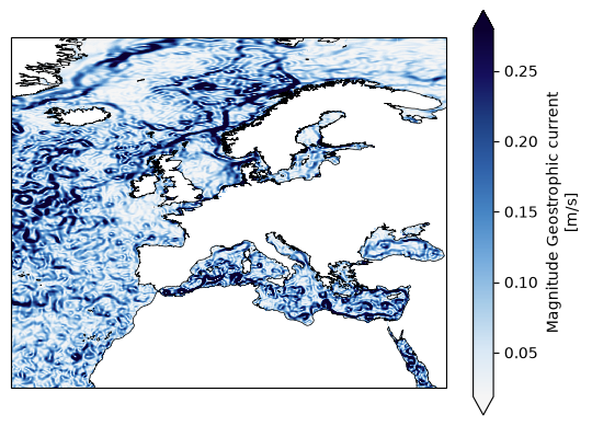
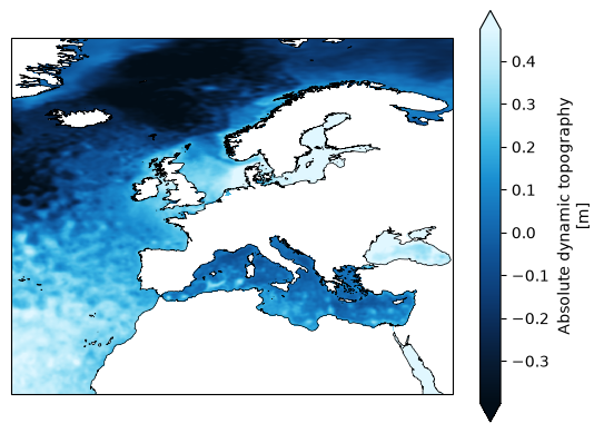
Gridded Sea Level Anomalies (SLA) from the application of the Multiscale Inversion of Ocean Surface Topography (MIOST) algorithm. This product provides additional variables such as Absolute Dynamic Topography and geostrophic currents (both absolute values and anomalies) at a resolution of 1/16° over the Europeans Seas and for the period from 2023-03-28 to 2024-12-31. It is intended for delayed-time applications.
Original Data Source: https://
zenodo .org /records /16793036 Reference: https://
opensciencedata .esa .int /products /coastdyn -adt -rep -2d -dataset /collection OSC entry: https://
opensciencedata .esa .int /products /coastdyn -adt -rep -2d -dataset /collection License: CC-BY-4.0
import xarray as xrds = xr.open_zarr('https://s3.waw4-1.cloudferro.com/EarthCODE/OSCAssets/coastdyn/coastdyn-miost-l4.zarr/')
dsLoading...
import matplotlib.pyplot as plt
from matplotlib.colors import LinearSegmentedColormap
import cartopy.crs as ccrs
import cartopy.feature as cfeature
from cartopy.mpl.gridliner import LONGITUDE_FORMATTER, LATITUDE_FORMATTER
import matplotlib.ticker as mticker
from matplotlib.colors import BoundaryNorm
import numpy as np
Select a date of interest
date = "2024-01-25"Read dataset & compute magnitude of the geostrophic current
da = ds.sel(time=np.datetime64(date), drop=True)
da['ugeo'] = np.sqrt(da.ugos**2 + da.vgos**2)
da['ugeo'].attrs['long_name'] = 'Magnitude Geostrophic current'
da['ugeo'].attrs['units'] = 'm/s'
da
Loading...
Plot Absolute Dynamic Topopgraphy example
bathymetry = ['#020d17', '#071a30', '#0a2a54', '#0d3f7a', '#0f5498', '#1570b8', '#1a8fd1', '#3bb5e3', '#7dd5f0', '#b8eaf9', '#e0f7ff']

# Create matplotlib colormap for adt
cmap_adt = LinearSegmentedColormap.from_list(
    'bathymetry', bathymetry
)


fig, axis = plt.subplots(1, 1, subplot_kw=dict(projection=ccrs.PlateCarree()))
da.adt.plot(cmap=cmap_adt,
            vmin=np.nanpercentile(da.adt, 5),
            vmax=np.nanpercentile(da.adt, 95),
            transform=ccrs.PlateCarree())
axis.coastlines(resolution='10m', lw=0.5)

# Longitude and latitude gridlines
# remove the gridlines code if you dont see the map.
gl = axis.gridlines(
    crs=ccrs.PlateCarree(),
    draw_labels=True,
    linewidth=0.5,
    color='gray',
    alpha=0.5,
    linestyle='--'
)

gl.top_labels = False
gl.right_labels = False

gl.xlocator = mticker.FixedLocator(np.arange(-180, 181, 30))
gl.ylocator = mticker.FixedLocator(np.arange(-90, 91, 15))

gl.xformatter = LONGITUDE_FORMATTER
gl.yformatter = LATITUDE_FORMATTER

gl.xlabel_style = {'size': 10}
gl.ylabel_style = {'size': 10}

plt.show()
Plot Magnitude of Geostrophic current
wind_speed = ['#f5f5f5', '#d9e8f5', '#a8cce8', '#74aadc', '#4685c4', '#2f60a8', '#1e3f82', '#150f5c', '#0b0030']

# Create matplotlib colormap for velocity
cmap_u = LinearSegmentedColormap.from_list(
    'wind-speed', wind_speed
)


fig, axis = plt.subplots(1, 1, subplot_kw=dict(projection=ccrs.PlateCarree()))
da.ugeo.plot(cmap=cmap_u,
            vmin=np.nanpercentile(da.ugeo, 5),
            vmax=np.nanpercentile(da.ugeo, 95),
            transform=ccrs.PlateCarree())
axis.coastlines(resolution='10m', lw=0.5)

# Longitude and latitude gridlines
# remove the gridlines code if you dont see the map.

gl = axis.gridlines(
    crs=ccrs.PlateCarree(),
    draw_labels=True,
    linewidth=0.5,
    color='gray',
    alpha=0.5,
    linestyle='--'
)

gl.top_labels = False
gl.right_labels = False

gl.xlocator = mticker.FixedLocator(np.arange(-180, 181, 30))
gl.ylocator = mticker.FixedLocator(np.arange(-90, 91, 15))

gl.xformatter = LONGITUDE_FORMATTER
gl.yformatter = LATITUDE_FORMATTER

gl.xlabel_style = {'size': 10}
gl.ylabel_style = {'size': 10}

plt.show()