Explore re-projected dataset in the Med cube
This product provides the Finite-size Lyapunov Exponents derived from surface geostrophic velocities result from the application of the MIOST algorithm (Ubelmann et al., 2019; Ubelmann et al. (2021)) to altimetry L3-data (Ballarotta & Verbrugge (2024)) at a resolution of 1/24° over the Mediterranean Sea and for the period from April 2016 to July 2022.
Original Data Source: https://
zenodo .org /records /11384073 Reference: Hernández-Carrasco et al. (2011)
OSC entry: https://
opensciencedata .esa .int /stac -browser / # /products /4dmed -2d -alt -miost -le -24 /collection .json License: CC-BY-4.0
import xarray as xr
import numpy as np
import pandas as pd
from pystac_client import Client

catalog = Client.open("https://eoapi.workspace.earthcode.eox.at/stac/")
item = next(catalog.search(collections=["4dmed-2d-alt-miost-le-24"]).items())
item
Loading...
item.assets["data"].hrefds = xr.open_dataset(item.assets["data"].href)
dsLoading...
import matplotlib.pyplot as plt
import cartopy.crs as ccrs
import cartopy.feature as cfeature

# Choose date
date = "2020-06-15"

# Select FSLE for that date
fsle_day = ds["fsle"].sel(time=date)

# 2-D coordinates
lon = ds["lon"]
lat = ds["lat"]

# Create map
fig = plt.figure(figsize=(12, 7))

ax = plt.axes(projection=ccrs.PlateCarree())

# Plot FSLE
pcm = ax.pcolormesh(
    lon,
    lat,
    fsle_day,
    transform=ccrs.PlateCarree(),
    shading="auto",
    cmap="viridis"
)

# Basemap features
ax.add_feature(cfeature.LAND, facecolor="lightgray")
ax.add_feature(cfeature.COASTLINE, linewidth=0.8)
ax.add_feature(cfeature.BORDERS, linewidth=0.5)


# Colourbar
cbar = plt.colorbar(
    pcm,
    ax=ax,
    orientation="vertical",
    pad=0.03,
    shrink=0.8
)
cbar.set_label("FSLE")

ax.set_title(f"FSLE - {date}")

plt.tight_layout()
plt.show()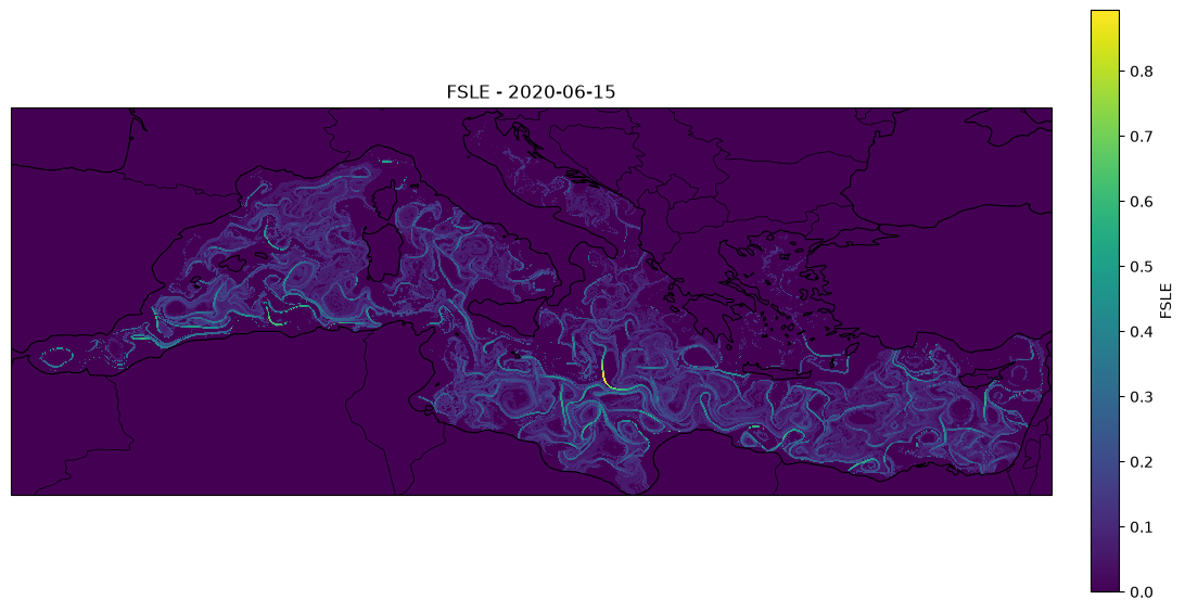
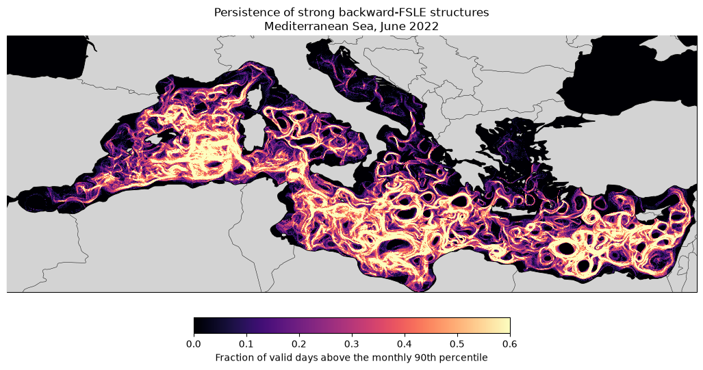
Find strong and persistent currents in June 2022
target_month = "2022-06"

fsle_month = ds.fsle.sel(time=target_month).compute()
strong_fsle = float(
fsle_month.quantile(
0.90,
dim=("time", "y", "x"),
skipna=True
)
)
print(f"Monthly 90th-percentile threshold: {strong_fsle:.3f} day⁻¹")Monthly 90th-percentile threshold: 0.100 day⁻¹
valid_days = fsle_month.notnull().sum("time")

persistence = (
    (fsle_month >= strong_fsle).sum("time") / valid_days
).where(valid_days > 0)

mean_fsle = fsle_month.mean("time", skipna=True)
mean_fsle
Loading...
# visualise

import matplotlib.pyplot as plt
import cartopy.crs as ccrs
import cartopy.feature as cfeature

projection = ccrs.PlateCarree()

fig = plt.figure(figsize=(13, 6))
ax = plt.axes(projection=projection)

mesh = ax.pcolormesh(
    ds.lon,
    ds.lat,
    persistence,
    transform=projection,
    shading="auto",
    cmap="magma",
    vmin=0,
    vmax=0.6
)

ax.add_feature(cfeature.LAND, facecolor="lightgray", zorder=3)
ax.add_feature(cfeature.COASTLINE, linewidth=0.6, zorder=4)
ax.add_feature(cfeature.BORDERS, linewidth=0.35, zorder=4)

colorbar = plt.colorbar(
    mesh,
    ax=ax,
    orientation="horizontal",
    pad=0.08,
    fraction=0.05
)

colorbar.set_label("Fraction of valid days above the monthly 90th percentile")

ax.set_title(
    "Persistence of strong backward-FSLE structures\n"
    "Mediterranean Sea, June 2022"
)
- Ubelmann, C., Dibarboure, G., Gaultier, L., Ponte, A., Ardhuin, F., Ballarotta, M., & Faugère, Y. (2021). Reconstructing Ocean Surface Current Combining Altimetry and Future Spaceborne Doppler Data. Journal of Geophysical Research: Oceans, 126(3). 10.1029/2020jc016560
- Ballarotta, M., & Verbrugge, N. (2024). ESA 4DMED-SEA - Mediterranean Sea Gridded MIOST L4 Sea Surface Heights And Derived Variables. Zenodo. 10.5281/ZENODO.10648981
- Hernández-Carrasco, I., López, C., Hernández-García, E., & Turiel, A. (2011). How reliable are finite-size Lyapunov exponents for the assessment of ocean dynamics? Ocean Modelling, 36(3–4), 208–218. 10.1016/j.ocemod.2010.12.006