This repository contains information and guided notebooks about the Ocean Hackathon. The core aspects of the hackathon are:
Marine datasets covering the Mediterranean Sea and the global ocean from ESA-funded science projects, hosted on object storage.
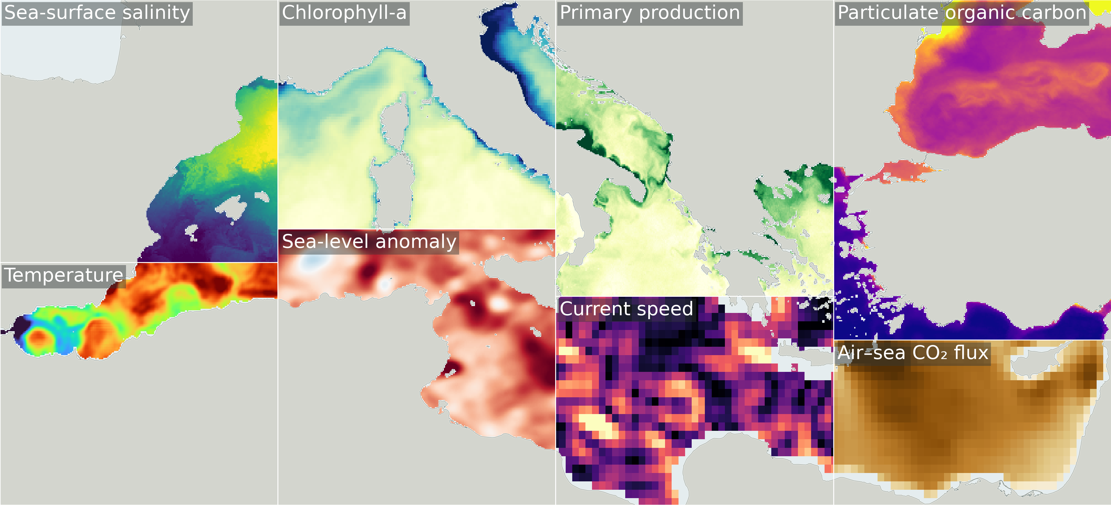
A Mediterranean Sea datacube with a common spatial grid and separate stores for monthly, hourly, and daily data.
Guided notebooks that show how to access the cloud-hosted datasets, convert data into cloud-native formats, combine them into analysis-ready datacubes, and use those collections in scientific workflows.
Information about creating a local environment to work in, or using the provided cloud platform.
Repository Map
| Folder | Purpose | Best starting point |
|---|---|---|
0_Introduction/ | Brief introduction to the hackathon, goals, EarthCODE context, setup, and agenda. | 0_Introduction/intro.ipynb |
1_Datasets/ | Dataset catalogue and information per source product. | 1_Datasets/datasets_sumary.ipynb |
2_Datacube/ | ESA Mediterranean Sea Datacube and access examples. | 2_Datacube/0_intro.ipynb |
3_File_formats_and_metadata/ | Format-conversion examples for Zarr, COG, and GeoParquet, plus the creation of STAC metadata. | 3_File_formats_and_metadata/0_intro.ipynb |
5_Hackathon_Code/ | Folder for your code. | 5_Hackathon_Code/0_intro.md |
Generated local data is expected in downloaded_data/, which is ignored by Git.
EarthCODE Context
The hackathon is supported by EarthCODE, and the data is available through EarthCODE’s Open Science Catalog.
1. Datasets prepared for the Ocean Hackathon
Each prepared dataset has an associated notebook, linked in the access notebook column, showing how to open its assets directly from object storage. More information about each dataset is available in its notebook and OSC entry. All notebooks reside in the 1_Datasets folder.
| Dataset | Description | Prepared format | CRS/grid | Time coverage | Licence | Links | Access notebook |
|---|---|---|---|---|---|---|---|
| 4DMED-SEA sea-surface salinity | Mediterranean salinity and density fields | Zarr | EPSG:4326, 1/24° lat/lon grid | Daily, 2016–2022 | CC-BY-4.0 | OSC | Notebook |
| 4DMED-SEA MIOST Lagrangian eddies | Mediterranean current structures and eddies | Zarr | EPSG:4326, 1/24° lat/lon grid | Daily, April 2016–July 2022 | CC-BY-4.0 | OSC | Notebook |
| 4DMED-SEA 4DVarNet 1/8° | Sea-level and geostrophic velocity fields | Zarr | EPSG:4326, 1/8° lat/lon grid | Daily, January 2016–August 2022 | CC-BY-4.0 | OSC | Notebook |
| 4DMED-SEA 4DVarNet 1/20° | Sea-surface height and derived variables | Zarr | EPSG:4326, 1/20° lat/lon grid | Daily, January 2016–August 2022 | CC-BY-4.0 | OSC | Notebook |
| 4DMED-SEA PFT and Kd | Phytoplankton functional types and diffuse attenuation | Zarr | EPSG:4326, 8 km lat/lon grid | Monthly, 2019–2021 | CC-BY-4.0 | OSC | Notebook |
| 4DMED-SEA 3D physical fields | Temperature, salinity, density, and geostrophic velocity | Zarr | EPSG:4326, 1/24° grid with 20 depth levels to 153 m | Daily, January 2016–July 2022 | CC-BY-4.0 | OSC | Notebook |
| 4DMED-SEA primary production | Primary production from chlorophyll and temperature | Zarr | EPSG:4326, 1/24° grid with 148 depth levels to 150 m | Daily, January 2016–August 2022 | CC-BY-4.0 | OSC | Notebook |
| 4DMED-SEA 3D biophysical fields | Chlorophyll-a plus physical and velocity variables | Zarr | EPSG:4326, 1/24° grid with 148 depth levels to 150 m | Daily, January 2016–August 2022 | CC-BY-4.0 | OSC | Notebook |
| WOC total surface current | Hourly total ocean current at 15 m | Zarr | EPSG:4326, 0.25° lat/lon grid at 15 m | Hourly, December 2014–December 2019 | CC-BY-4.0 | OSC | Notebook |
| Atlantic Ocean heat content | Atlantic heat-content change | Zarr | EPSG:4326, global 1° lat/lon grid | April 2002–September 2023 | AVISO terms | OSC | Notebook |
| OceanSODA-ETHZ | Surface-ocean carbonate-system variables | Zarr | EPSG:4326, global 1° and 0.25° lat/lon grids | Monthly, 1982–2024; 8-day products, 1982–2022 | CC-BY-NC-SA-4.0 | OSC | Notebook |
| WAPOSAL | Wave and satellite-altimetry products | Zarr | EPSG:4326, along-track observations | March 2016–December 2022 | CC-BY-SA-4.0 | OSC | Notebook |
| MITHO | Global cumulative hazard indexes | Zarr | EPSG:4326, global 1° lat/lon grid | Monthly; varies by index, 1993–2022 | CC-BY-SA-4.0 | OSC | Notebook |
| BICEP | Biological pump and carbon exchange processes | Zarr | EPSG:4326, global regular lat/lon grids | Monthly, 1997–2020 | UK Open Government Licence | OSC | Notebook |
| CAREHeat | Marine heat waves | Zarr | EPSG:4326, global 0.25° lat/lon grid | Daily, 1980–2024 | CC-BY-4.0 | OSC | Notebook |
| Booms | Biodiversity in the Open Ocean: Mapping, Monitoring and Modelling (BOOMS) | Zarr | EPSG:4326, global 0.04° lat/lon grid | Daily, 1998–2024 | CC-BY-NC-4.0 | OSC | Notebook |
| CoastDyn | ESA COASTDyn | Zarr | EPSG:4326, Europe 0.0625° lat/lon grid | Daily, 2023-2024 | CC-BY-4.0 | OSC | Notebook |
2. ESA Mediterranean Sea Datacube
The ESA Mediterranean Sea Datacube combines marine datasets on a common 1/24° EPSG:4326 grid. The data are available in four online GeoZarr stores with different time and depth coordinates:
| Store | Contents | Cube coordinate coverage |
|---|---|---|
| ocean | 4DMED PFT/Kd, ocean heat content, OceanSODA, BICEP, and MITHO | Monthly, January 2016–December 2022 |
| hourly_cube.zarr | WOC and CMEMS current components at 15 m | Hourly, 30 December 2014–30 December 2019 |
| ocean | 4DMED primary production and 3D physical fields at 18 depths, 3–135 m | Daily, 1 January 2016–31 July 2022 |
| ocean | 4DMED salinity/density, FSLE, both 4DVarNet reconstructions, and CAREHeat categories | Daily, 1 January 2016–31 December 2022 |
The notebooks open these online stores directly over HTTPS using consolidated metadata. An internet connection is required; only the selected chunks are read. Group 0 is full resolution; groups 1 and 2 contain spatial summaries at 1/6° and 1/3°. Individual products may cover only part of a store’s time axis.
Start with cube access and example plots, then explore building a small local cube and time series at every depth. The overview lists source products, OSC links, variables, licences, and how the data were combined.
3. File Formats and Metadata
The format notebooks show 1) how datasets can be transformed in cloud-optimised formats, and 2) described with metadata.
Note: the examples we used for these notebooks come from Polar studies, since they came in different file formats.
Dataset Formats
| Format | Best for | Why it matters in object storage |
|---|---|---|
| Zarr | Labelled multidimensional arrays | Chunked reads allow an analysis to load only the required variables, regions, depths, and times. |
| Cloud Optimized GeoTIFF (COG) | Individual rasters or raster stacks | Internal tiling and overviews support efficient range reads and quicklooks. |
| GeoParquet | Vector geometries and tabular observations | Columnar storage enables efficient filtering and carries standard geospatial metadata. |
See the notebooks in 3_File_formats_and_metadata/ and the Cloud-Native Geospatial Guide for more detail.
Metadata
Rich metadata makes each collection easier to find, interpret, cite, and reuse. Collection metadata should document provenance, licence, variables, units, spatial and temporal extent, processing history, and access assets.
EarthCODE collections use the SpatioTemporal Asset Catalog (STAC) specification to provide a consistent, machine-readable description of geospatial data.
4. Visualisation
Most of the datasets are part of one of the cubes, which in turn can be interactively visualised since they are in geozarr format. To open the visualisation click the “Explore Data” link in the ntoebooks, or go directly to the visualisation website . The site wraps a simple GeoZarr viewer and can be replaced with a compatible GeoZarr in any programming language or tool. Additionally, there are two notebooks if you are interested in converting your own data. They use a sample of the OceanSoda Dataset to demonstrate the conversions:
Suggested Hackathon Workflow
Pick a science question, user workflow, or define your own.
Browse the dataset catalogue and open the relevant access notebooks.
Use the existing collections to answer the question.
Use the file-format notebooks as guidance when preparing a new dataset to add to the existing collections.
Put your code in
5_Hackathon_Code/and keep generated data out of Git.Submit your work as a pull request with a short description of the question, datasets, methods, and outputs.
Environment Notes
The notebooks assume a Python geospatial environment with common Pangeo tools. The repository’s pixi.toml provides packages including xarray, dask, geopandas, rasterio, rioxarray, pyproj, shapely, pandas, numpy, matplotlib, and pystac.
Install the environment and start JupyterLab with:
pixi install
pixi run jupyter lab
Network access is only needed for remote object-store reads or optional source downloads. The format tutorials write generated examples to downloaded_data/, which is ignored by Git.