Access 4DMED-SEA 4DVarNet 1/20°

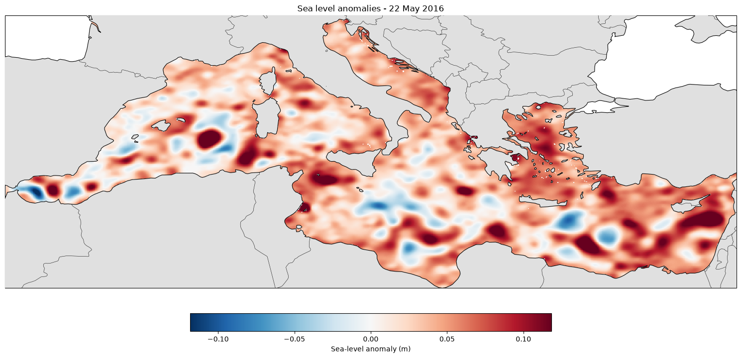
* Original Data Source: zenodo.org/records/10912777
* Reference:  https://doi.org/10.3390/rs14102502
* OSC entry: https://opensciencedata.esa.int/stac-browser/#/products/4dmed-2d-alt-varnet-20/collection.json
* License: CC-BY-4.0

import xarray as xr

zarr_href = 'https://s3.waw4-1.cloudferro.com/EarthCODE/OSCAssets/ocean_datasets/4dvarnet-ssh.zarr/'

ds = xr.open_zarr(zarr_href)
ds

snapshot = ds.sel(time="2016-05-22")
snapshot

import numpy as np

sla_limit = float(np.nanpercentile(np.abs(snapshot.sla), 98))

import matplotlib.pyplot as plt
import matplotlib.lines as mlines
import cartopy.crs as ccrs
import cartopy.feature as cfeature

fig = plt.figure(figsize=(15, 8))
ax = plt.axes(projection=ccrs.PlateCarree())

ax.set_extent([
    float(snapshot.longitude.min()),
    float(snapshot.longitude.max()),
    float(snapshot.latitude.min()),
    float(snapshot.latitude.max())
], crs=ccrs.PlateCarree())

# Plot SLA with limits centred on zero so positive and negative anomalies are comparable
sla_plot = ax.pcolormesh(
    snapshot.longitude,
    snapshot.latitude,
    snapshot.sla,
    cmap="RdBu_r",
    vmin=-sla_limit,
    vmax=sla_limit,
    shading="auto",
    transform=ccrs.PlateCarree()
)

# Add coastlines and land to provide geographic context
ax.add_feature(cfeature.LAND, facecolor="0.88", zorder=3)
ax.coastlines(resolution="50m", linewidth=0.8, zorder=4)
ax.add_feature(cfeature.BORDERS, linewidth=0.4, zorder=4)


# Explain the SLA colours and vorticity contour meanings
colorbar = plt.colorbar(
    sla_plot,
    ax=ax,
    orientation="horizontal",
    pad=0.07,
    fraction=0.05
)
colorbar.set_label("Sea-level anomaly (m)")


ax.set_title(
    "Sea level anomalies - 22 May 2016"
)

plt.tight_layout()
plt.show()