Original Data Source: https://
zenodo .org /records /16793036 Reference: https://
opensciencedata .esa .int /products /coastdyn -adt -rep -2d -dataset /collection OSC entry: https://
opensciencedata .esa .int /products /coastdyn -adt -rep -2d -dataset /collection License: CC-BY-4.0
import xarray as xrds = xr.open_zarr('https://s3.waw4-1.cloudferro.com/EarthCODE/OSCAssets/coastdyn/coastdyn-miost-l4.zarr/')
dsLoading...
import matplotlib.pyplot as plt
from matplotlib.colors import LinearSegmentedColormap
import cartopy.crs as ccrs
import cartopy.feature as cfeature
from cartopy.mpl.gridliner import LONGITUDE_FORMATTER, LATITUDE_FORMATTER
import matplotlib.ticker as mticker
from matplotlib.colors import BoundaryNorm
import numpy as np
Select a date of interest
date = "2024-01-25"Read dataset & compute magnitude of the geostrophic current
da = ds.sel(time=np.datetime64(date), drop=True)
da['ugeo'] = np.sqrt(da.ugos**2 + da.vgos**2)
da['ugeo'].attrs['long_name'] = 'Magnitude Geostrophic current'
da['ugeo'].attrs['units'] = 'm/s'
da
Loading...
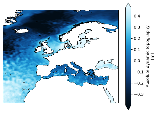
Plot Absolute Dynamic Topopgraphy example
bathymetry = ['#020d17', '#071a30', '#0a2a54', '#0d3f7a', '#0f5498', '#1570b8', '#1a8fd1', '#3bb5e3', '#7dd5f0', '#b8eaf9', '#e0f7ff']

# Create matplotlib colormap for adt
cmap_adt = LinearSegmentedColormap.from_list(
    'bathymetry', bathymetry
)


fig, axis = plt.subplots(1, 1, subplot_kw=dict(projection=ccrs.PlateCarree()))
da.adt.plot(cmap=cmap_adt,
            vmin=np.nanpercentile(da.adt, 5),
            vmax=np.nanpercentile(da.adt, 95),
            transform=ccrs.PlateCarree())
axis.coastlines(resolution='10m', lw=0.5)

# Longitude and latitude gridlines
# remove the gridlines code if you dont see the map.
gl = axis.gridlines(
    crs=ccrs.PlateCarree(),
    draw_labels=True,
    linewidth=0.5,
    color='gray',
    alpha=0.5,
    linestyle='--'
)

gl.top_labels = False
gl.right_labels = False

gl.xlocator = mticker.FixedLocator(np.arange(-180, 181, 30))
gl.ylocator = mticker.FixedLocator(np.arange(-90, 91, 15))

gl.xformatter = LONGITUDE_FORMATTER
gl.yformatter = LATITUDE_FORMATTER

gl.xlabel_style = {'size': 10}
gl.ylabel_style = {'size': 10}

plt.show()
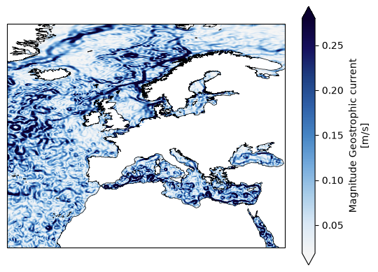
Plot Magnitude of Geostrophic current
wind_speed = ['#f5f5f5', '#d9e8f5', '#a8cce8', '#74aadc', '#4685c4', '#2f60a8', '#1e3f82', '#150f5c', '#0b0030']

# Create matplotlib colormap for velocity
cmap_u = LinearSegmentedColormap.from_list(
    'wind-speed', wind_speed
)


fig, axis = plt.subplots(1, 1, subplot_kw=dict(projection=ccrs.PlateCarree()))
da.ugeo.plot(cmap=cmap_u,
            vmin=np.nanpercentile(da.ugeo, 5),
            vmax=np.nanpercentile(da.ugeo, 95),
            transform=ccrs.PlateCarree())
axis.coastlines(resolution='10m', lw=0.5)

# Longitude and latitude gridlines
# remove the gridlines code if you dont see the map.

gl = axis.gridlines(
    crs=ccrs.PlateCarree(),
    draw_labels=True,
    linewidth=0.5,
    color='gray',
    alpha=0.5,
    linestyle='--'
)

gl.top_labels = False
gl.right_labels = False

gl.xlocator = mticker.FixedLocator(np.arange(-180, 181, 30))
gl.ylocator = mticker.FixedLocator(np.arange(-90, 91, 15))

gl.xformatter = LONGITUDE_FORMATTER
gl.yformatter = LATITUDE_FORMATTER

gl.xlabel_style = {'size': 10}
gl.ylabel_style = {'size': 10}

plt.show()