Access BICEP - Ocean Hackathon

* Original Data Source: https://data.ceda.ac.uk/neodc/bicep/data
* Reference:  https://opensciencedata.esa.int/projects/biological-pump-and-carbon-exchange-processes/collection
* OSC entry: https://opensciencedata.esa.int/projects/biological-pump-and-carbon-exchange-processes/collection , https://opensciencedata.esa.int/products/bicep-database/collection.json
* License: Open Data License (UK Gov)

import xarray as xr

zarr_href1 = 'https://s3.waw4-1.cloudferro.com/EarthCODE/OSCAssets/ocean_datasets/bicep_marine_primary_productivity.zarr/'
zarr_href2 = 'https://s3.waw4-1.cloudferro.com/EarthCODE/OSCAssets/ocean_datasets/bicep_oceanic_export_production.zarr/'
zarr_href3 = 'https://s3.waw4-1.cloudferro.com/EarthCODE/OSCAssets/ocean_datasets/particulate_organic_carbon_geo.zarr'
zarr_href4 = 'https://s3.waw4-1.cloudferro.com/EarthCODE/OSCAssets/ocean_datasets/phytoplankton_carbon.zarr/'

zarr_href1 = '/run/media/krasen/Storage/ocean/processed/bicep/bicep_marine_primary_productivity.zarr/'
zarr_href2 = '/run/media/krasen/Storage/ocean/processed/bicep/bicep_oceanic_export_production.zarr/'
zarr_href3 = '/run/media/krasen/Storage/ocean/processed/bicep/particulate_organic_carbon_geo.zarr'
zarr_href4 = '/run/media/krasen/Storage/ocean/processed/bicep/phytoplankton_carbon.zarr/'

ds = xr.open_zarr(zarr_href3)
ds

marine primary productivity¶

ds = xr.open_zarr(zarr_href1)
ds

import matplotlib.pyplot as plt
import cartopy.crs as ccrs
import cartopy.feature as cfeature
import numpy as np

# Choose date
date = "2020-06"

# Select FSLE for that date
pp = ds["pp"].sel(time=np.datetime64(date), lon=slice(-6.062, 36.06), lat=slice(30.27, 45.98), drop=True)


# 2-D coordinates
lon = pp["lon"]
lat = pp["lat"]

# Create map
fig = plt.figure(figsize=(12, 7))

ax = plt.axes(projection=ccrs.PlateCarree())

# Plot FSLE
pcm = ax.pcolormesh(
    lon,
    lat,
    pp,
    transform=ccrs.PlateCarree(),
    shading="auto",
    cmap="viridis"
)

# Basemap features
ax.add_feature(cfeature.LAND, facecolor="lightgray")
ax.add_feature(cfeature.COASTLINE, linewidth=0.8)
ax.add_feature(cfeature.BORDERS, linewidth=0.5)



# Colourbar
cbar = plt.colorbar(
    pcm,
    ax=ax,
    orientation="vertical",
    pad=0.03,
    shrink=0.8
)
cbar.set_label("PP")

ax.set_title(f"gross_primary_production_of_carbon (mg C m-2 d-1) — {date}")

plt.tight_layout()
plt.show()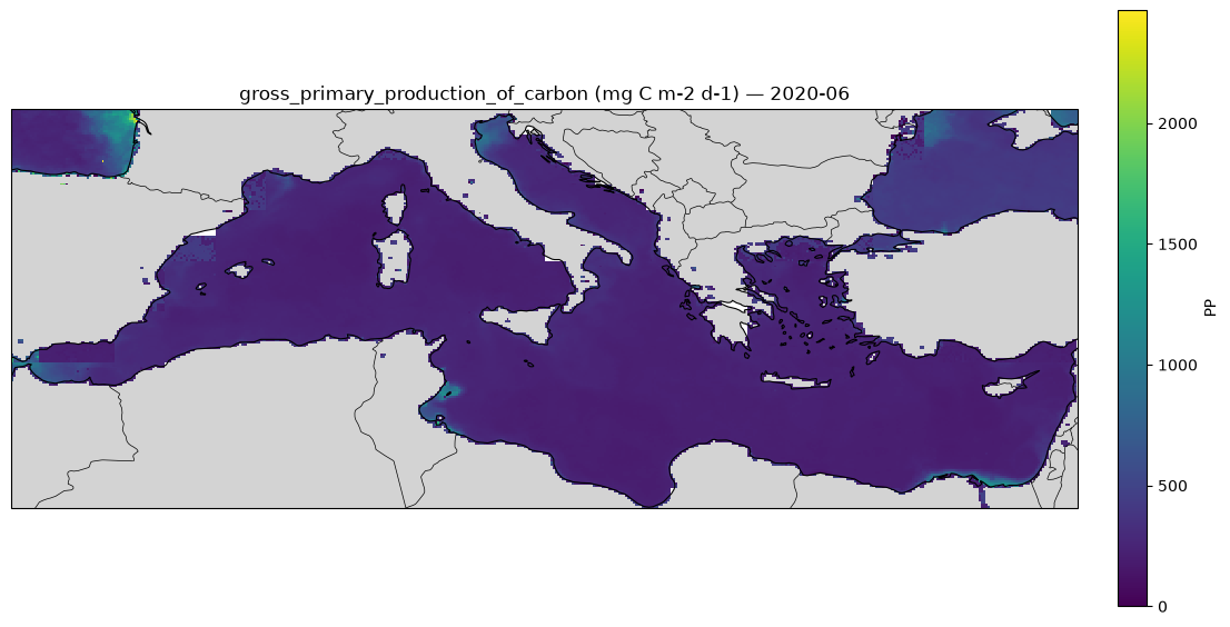

Export Productivity¶

ds = xr.open_zarr(zarr_href2)
ds

import matplotlib.pyplot as plt
import cartopy.crs as ccrs
import cartopy.feature as cfeature

# Select June 2016
# Your timestamps appear to be monthly, e.g. 2016-06-16
ds_june = ds.sel(time="2020-06").squeeze("time")

variables = ["EP_Dunne", "EP_Henson", "EP_Li"]

fig, axes = plt.subplots(
    nrows=3,
    ncols=1,
    figsize=(12, 12),
    subplot_kw={"projection": ccrs.PlateCarree()},
    constrained_layout=True
)

for ax, var in zip(axes, variables):

    da = ds_june[var]

    im = ax.pcolormesh(
        ds_june.lon,
        ds_june.lat,
        da,
        transform=ccrs.PlateCarree(),
        shading="auto",
        cmap="viridis"
    )

    ax.coastlines()
    ax.add_feature(cfeature.LAND, facecolor="lightgray")
    ax.set_global()


    ax.set_title(
        f"{da.attrs.get('description', var)} — June 2016",
        fontsize=12
    )

    cbar = fig.colorbar(
        im,
        ax=ax,
        orientation="vertical",
        pad=0.02,
        shrink=0.8
    )
    cbar.set_label("mg C m$^{-2}$ d$^{-1}$")

plt.show()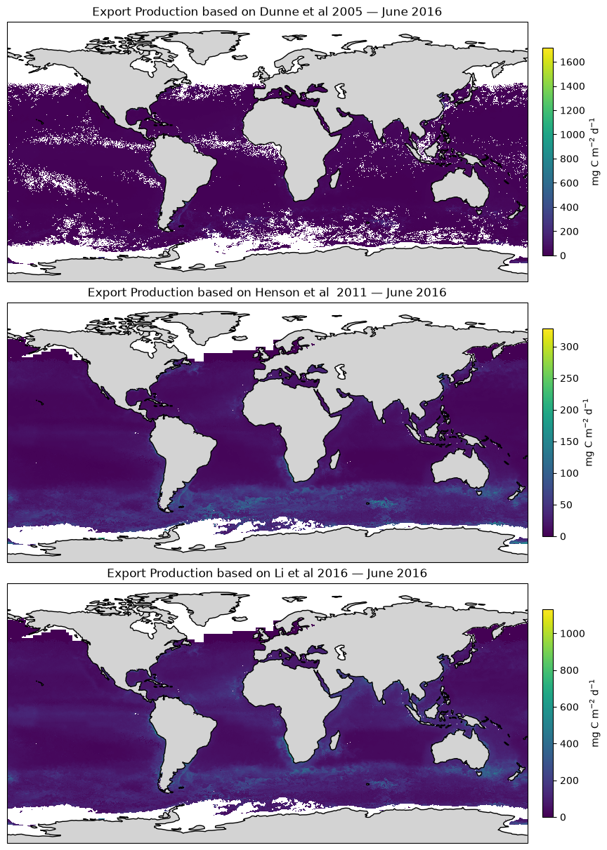

particulate_organic_carbon_geo¶

ds = xr.open_zarr(zarr_href3)
ds

import matplotlib.pyplot as plt
import cartopy.crs as ccrs
import cartopy.feature as cfeature
import numpy as np

# Choose date
date = "2020-06"

# Select FSLE for that date
pp = ds["POC"].sel(time=np.datetime64(date), lon=slice(-6.062, 36.06), lat=slice(45.98, 30.27,), drop=True)


# 2-D coordinates
lon = pp["lon"]
lat = pp["lat"]

# Create map
fig = plt.figure(figsize=(12, 7))

ax = plt.axes(projection=ccrs.PlateCarree())

# Plot FSLE
pcm = ax.pcolormesh(
    lon,
    lat,
    pp,
    transform=ccrs.PlateCarree(),
    shading="auto",
    cmap="viridis"
)

# Basemap features
ax.add_feature(cfeature.LAND, facecolor="lightgray")
ax.add_feature(cfeature.COASTLINE, linewidth=0.8)
ax.add_feature(cfeature.BORDERS, linewidth=0.5)



# Colourbar
cbar = plt.colorbar(
    pcm,
    ax=ax,
    orientation="vertical",
    pad=0.03,
    shrink=0.8
)
cbar.set_label("Particulate Organic Carbon")

ax.set_title(f"Particulate Organic Carbon (mg m^-3) — {date}")

plt.tight_layout()
plt.show()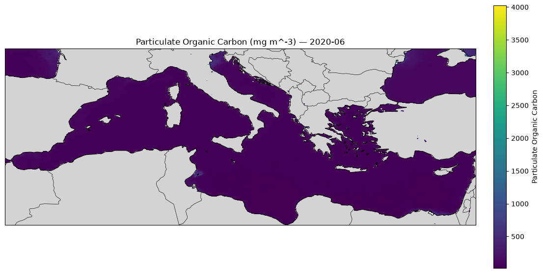

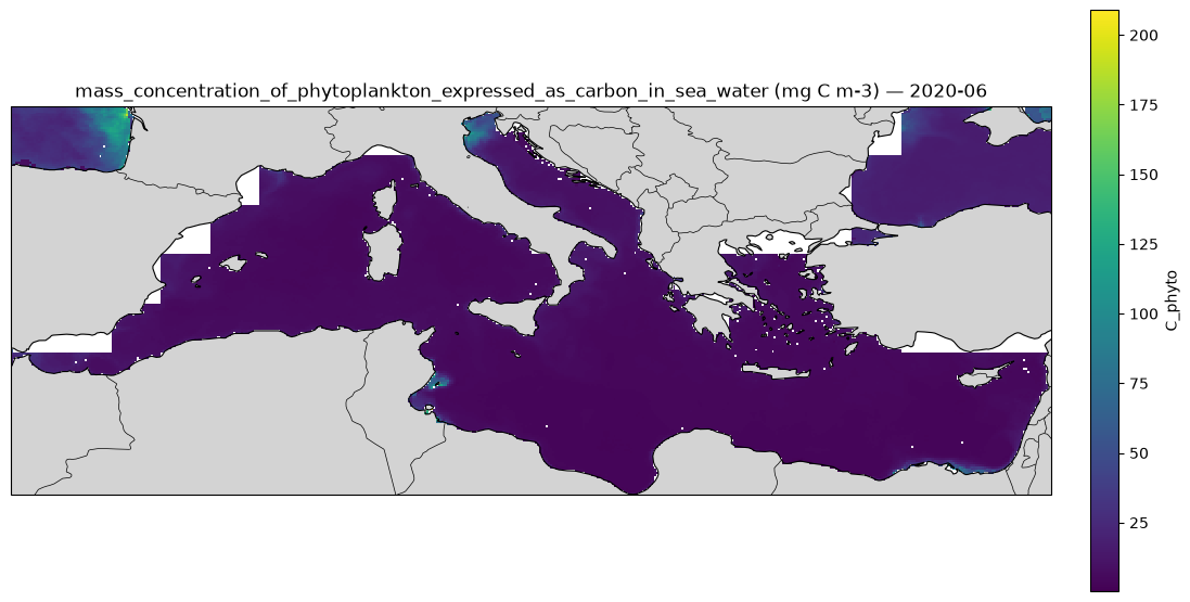
phytoplankton_carbon¶

ds = xr.open_zarr(zarr_href4)
ds

import matplotlib.pyplot as plt
import cartopy.crs as ccrs
import cartopy.feature as cfeature
import numpy as np

# Choose date
date = "2020-06"

# Select FSLE for that date
pp = ds["C_phyto"].sel(time=np.datetime64(date), lon=slice(-6.062, 36.06), lat=slice(30.27,45.98), drop=True)


# 2-D coordinates
lon = pp["lon"]
lat = pp["lat"]

# Create map
fig = plt.figure(figsize=(12, 7))

ax = plt.axes(projection=ccrs.PlateCarree())

# Plot FSLE
pcm = ax.pcolormesh(
    lon,
    lat,
    pp,
    transform=ccrs.PlateCarree(),
    shading="auto",
    cmap="viridis"
)

# Basemap features
ax.add_feature(cfeature.LAND, facecolor="lightgray")
ax.add_feature(cfeature.COASTLINE, linewidth=0.8)
ax.add_feature(cfeature.BORDERS, linewidth=0.5)



# Colourbar
cbar = plt.colorbar(
    pcm,
    ax=ax,
    orientation="vertical",
    pad=0.03,
    shrink=0.8
)
cbar.set_label("C_phyto")

ax.set_title(f"mass_concentration_of_phytoplankton_expressed_as_carbon_in_sea_water (mg C m-3) — {date}")

plt.tight_layout()
plt.show()