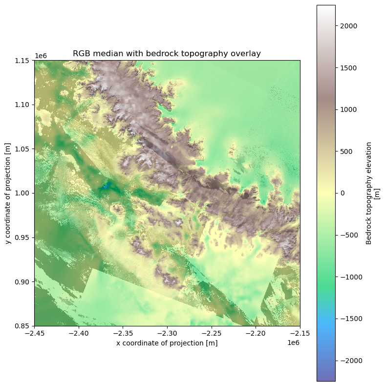
Accessing Sentinel-2 Data - Polar Hackathon

This notebook shows a simple end-to-end workflow for bringing Sentinel-2 L2A data into the Antarctic datacube workflow. We use the cube grid to define an area of interest, search a STAC API, load RGB and scene classification data lazily with odc.stac, build a least-bad-pixel mosaic, and plot polar cube data over the result.

import numpy as np
import warnings
import xarray as xr
from dask.array.core import PerformanceWarning
from dask.diagnostics import ProgressBar
from matplotlib.colors import BoundaryNorm, ListedColormap
from matplotlib.patches import Rectangle
from pyproj import Transformer
import jupyter_bokeh

import rioxarray as rxr
import matplotlib.pyplot as plt
import cartopy.crs as ccrs

from pystac_client import Client as pystac_client
from odc.stac import stac_load

warnings.filterwarnings("ignore", message="In a future version of xarray the default value for join.*", category=FutureWarning)
warnings.filterwarnings("ignore", message="Increasing number of chunks.*", category=PerformanceWarning)

from shapely.geometry import mapping, box, shape


# Approximate EPSG:3031 location for Palmer Land / George VI Ice Shelf.
ROI_CENTER_XY_M = (-2_300_000.0, 1000_000.0)
ROI_HALF_WIDTH_CELLS = 1500
CUBE_RES_M = 100

cx, cy = ROI_CENTER_XY_M
half = ROI_HALF_WIDTH_CELLS * CUBE_RES_M


antarctic_crs = ccrs.SouthPolarStereo(
    central_longitude=0,
    true_scale_latitude=-71,
)

Define the search area from the cube grid¶

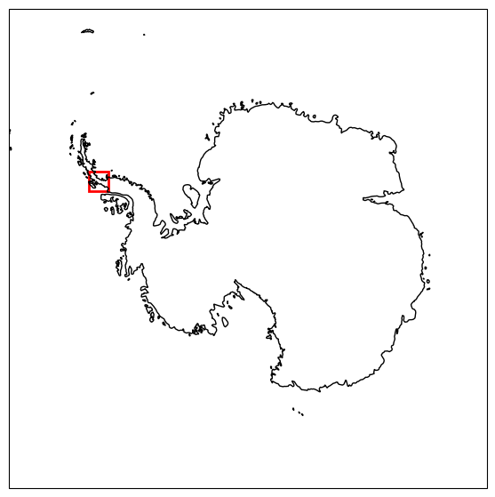
STAC searches expect longitude/latitude bounds, but our analysis area is easier to describe in the cube CRS. Here we define the ROI in EPSG:3031 metres, then transform its four corners to EPSG:4326 for the STAC bbox.

to_lonlat = Transformer.from_crs("EPSG:3031", "EPSG:4326", always_xy=True)

corners_3031 = [
    (cx - half, cy - half),
    (cx - half, cy + half),
    (cx + half, cy - half),
    (cx + half, cy + half),
]

corners_lonlat = [to_lonlat.transform(x, y) for x, y in corners_3031]

bbox = [
    min(lon for lon, lat in corners_lonlat),
    min(lat for lon, lat in corners_lonlat),
    max(lon for lon, lat in corners_lonlat),
    max(lat for lon, lat in corners_lonlat),
]

bbox

[-70.86635679409451,
 -68.95219601061162,
 -61.85839876773828,
 -65.45764355045239]

# Convert ROI center from meters to the appropriate scale and calculate half-width
cx, cy = ROI_CENTER_XY_M
half = ROI_HALF_WIDTH_CELLS * 100 

fig, ax = plt.subplots(figsize=(7, 7), subplot_kw={"projection": ccrs.SouthPolarStereo()})
ax.set_extent([-180, 180, -90, -58], crs=ccrs.PlateCarree())
ax.coastlines()
ax.add_patch(Rectangle((cx - half, cy - half), 2 * half, 2 * half, fill=False, edgecolor="red", linewidth=2, transform=ax.projection))
plt.show()

cube_paths = [
    "https://s3.waw4-1.cloudferro.com/EarthCODE/OSCAssets/antarctica_cube/icetemp.zarr",
    "https://s3.waw4-1.cloudferro.com/EarthCODE/OSCAssets/antarctica_cube/sec.zarr",
    "https://s3.waw4-1.cloudferro.com/EarthCODE/OSCAssets/antarctica_cube/antarctica-combined.zarr",
    "https://s3.waw4-1.cloudferro.com/EarthCODE/OSCAssets/antarctica_cube/icemask_composite.zarr/",
    "https://s3.waw4-1.cloudferro.com/EarthCODE/OSCAssets/antarctica_cube/ice_velocity.zarr",
]

ds = xr.open_mfdataset(cube_paths, engine="zarr", chunks={}, compat="no_conflicts")

x_index = int(np.abs(ds["x"].values - ROI_CENTER_XY_M[0]).argmin())
y_index = int(np.abs(ds["y"].values - ROI_CENTER_XY_M[1]).argmin())
x_slice = slice(x_index - ROI_HALF_WIDTH_CELLS, x_index + ROI_HALF_WIDTH_CELLS + 1)
y_slice = slice(y_index - ROI_HALF_WIDTH_CELLS, y_index + ROI_HALF_WIDTH_CELLS + 1)

ds = ds.isel(x=x_slice, y=y_slice).chunk({"x": -1, "y": -1})

ds

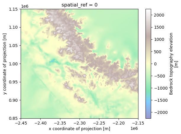
bed = ds.bedrock_topography_bed
bed_overlay = bed.where(bed.notnull() & (bed != 0))

bed_overlay.plot(
    x="x",
    y="y",
    cmap="terrain",
    alpha=0.5,
    add_colorbar=True,
)

Sentinel-2 Data Archives Access Example¶

Sentinel-2 L2A is the surface reflectance product and includes the scl scene classification layer used for masking clouds, shadows, nodata, and defective pixels.

catalog = pystac_client.open("https://earth-search.aws.element84.com/v1")
chunk={} # <-- use dask
res=100 # 100m resolution

query1 = catalog.search(
    collections=["sentinel-2-l2a"], datetime="2021-03-01/2021-03-30", limit=100, # sentinel-2-pre-c1-l2a
    bbox=bbox, query={"eo:cloud_cover": {"lt": 50}}
)

items = list(query1.items())
len(items)

84

Quick thumbnail check¶

The cloud-cover property is attached to the Sentinel-2 tile, not just the small ROI. A quick thumbnail pass is useful for spotting obviously bad acquisitions before loading the full data.

from IPython.display import Image, display
import ipywidgets as widgets

def show(i):
    item = items[i]
    print(i, item.id, item.properties.get("eo:cloud_cover"))
    display(Image(url=item.assets["thumbnail"].href, width=600))

widgets.interact(
    show,
    i=widgets.IntSlider(0, 0, len(items) - 1, continuous_update=False),
)

<function __main__.show(i)>

Load RGB and SCL onto the cube CRS¶

groupby="solar_day" combines same-day Sentinel-2 tiles into one time step. This matters because a large Antarctic bbox often intersects many MGRS tiles from the same pass. The data are loaded at 100 m to match the cube-scale workflow.

sen2_ds = stac_load(
    items,
    bands=("red", "green", "blue", 'scl'),
    crs="EPSG:3031",        # important: one common Antarctic grid
    resolution=100,
    bbox=bbox,
    chunks={},
    groupby="solar_day",
)

with ProgressBar():
    sen2_ds = sen2_ds.load()

sen2_ds

[########################################] | 100% Completed | 94.43 ss

Rank scenes by usable pixels¶

Masks bad Sentinel-2 pixels using scl.
Sorts the images by how many good pixels they have.
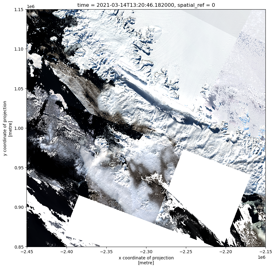
Builds an RGB mosaic by filling gaps with the next-best image, then reprojects it to match ds.

bad_scl = [0, 1, 3, 7, 8, 10]
# keep 11 = snow/ice ; leave 9 as well

clear = ~sen2_ds["scl"].isin(bad_scl)
clear_fraction = clear.mean(("x", "y")).compute()
clear_fraction.to_series().sort_values(ascending=False).head(10)


best_to_worst = clear_fraction.sortby(clear_fraction, ascending=False)["time"]

rgb_clear = sen2_ds[["red", "green", "blue"]].where(clear)
rgb_sorted = rgb_clear.sel(time=best_to_worst)

with ProgressBar():
    rgb_mosaic = rgb_sorted.bfill("time").isel(time=0).compute()

rgb_mosaic = rgb_mosaic.rio.reproject_match(ds)

Plot Sentinel Data Mosaic¶

rgb_da = rgb_mosaic.to_array("band")

rgb_da.plot.imshow(
    x="x",
    y="y",
    rgb="band",
    vmin=0,
    vmax=10000,
    figsize=(10, 10),
)

Overlay Bedrock Topography on Sentinel-2¶

fig, ax = plt.subplots(figsize=(8, 8))
rgb_da.plot.imshow(
    x="x",
    y="y",
    rgb="band",
    vmin=0,
    vmax=10000,
    ax=ax,
    add_colorbar=False,
)

bed_overlay.plot(
    x="x",
    y="y",
    ax=ax,
    cmap="terrain",
    alpha=0.7,
    add_colorbar=True,
)

ax.set_title("RGB median with bedrock topography overlay")
ax.set_aspect("equal")

plt.tight_layout()
plt.show()