Example ERA5 data access without a cloud account. It opens the public ARCO ERA5 Zarr archive on Google Cloud anonymously, uses full-resolution level 0 of the Antarctica land-ice GeoZarr for the analysis grid, subsets an Antarctic bbox, and plots 2 m air temperature.
Official sources:
ERA5 on the Copernicus Climate Data Store: https://
cds .climate .copernicus .eu /datasets /reanalysis -era5 -single -levels ECMWF ERA5 data documentation: https://
confluence .ecmwf .int /spaces /CKB /pages /76414402 /ERA5+data+documentation Google Cloud public datasets page: https://
docs .cloud .google .com /storage /docs /public -datasets Google Research ARCO ERA5 access examples: https://
github .com /google -research /arco -era5
import fsspec
import numpy as np
import warnings
import xarray as xr
from dask.array.core import PerformanceWarning
from dask.diagnostics import ProgressBar
from matplotlib.colors import BoundaryNorm, ListedColormap
from matplotlib.patches import Rectangle
from pyproj import Transformer
import jupyter_bokeh

import rioxarray as rxr
import matplotlib.pyplot as plt
import cartopy.crs as ccrs

from pystac_client import Client as pystac_client
from odc.stac import stac_load

warnings.filterwarnings("ignore", message="In a future version of xarray the default value for join.*", category=FutureWarning)
warnings.filterwarnings("ignore", message="Increasing number of chunks.*", category=PerformanceWarning)

from shapely.geometry import mapping, box, shape


# Approximate EPSG:3031 location for Palmer Land / George VI Ice Shelf.
ROI_CENTER_XY_M = (-2_300_000.0, 1000_000.0)
ROI_HALF_WIDTH_CELLS = 4000
CUBE_RES_M = 100

cx, cy = ROI_CENTER_XY_M
half = ROI_HALF_WIDTH_CELLS * CUBE_RES_M


antarctic_crs = ccrs.SouthPolarStereo(
    central_longitude=0,
    true_scale_latitude=-71,
)
to_lonlat = Transformer.from_crs("EPSG:3031", "EPSG:4326", always_xy=True)
corners_3031 = [
(cx - half, cy - half),
(cx - half, cy + half),
(cx + half, cy - half),
(cx + half, cy + half),
]
corners_lonlat = [to_lonlat.transform(x, y) for x, y in corners_3031]
bbox = [
min(lon for lon, lat in corners_lonlat),
min(lat for lon, lat in corners_lonlat),
max(lon for lon, lat in corners_lonlat),
max(lat for lon, lat in corners_lonlat),
]
bbox[-77.47119229084849,
-71.81000215448617,
-53.615648184164115,
-62.52573259978129]# Convert ROI center from meters to the appropriate scale and calculate half-width
cx, cy = ROI_CENTER_XY_M
half = ROI_HALF_WIDTH_CELLS * 100
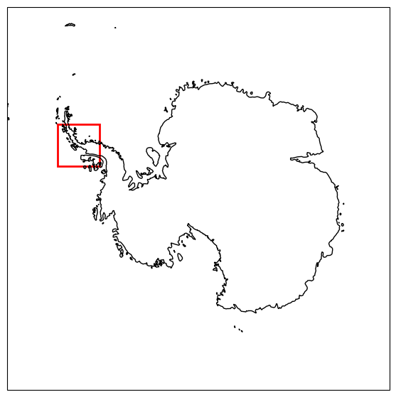
fig, ax = plt.subplots(figsize=(7, 7), subplot_kw={"projection": ccrs.SouthPolarStereo()})
ax.set_extent([-180, 180, -90, -58], crs=ccrs.PlateCarree())
ax.coastlines()
ax.add_patch(Rectangle((cx - half, cy - half), 2 * half, 2 * half, fill=False, edgecolor="red", linewidth=2, transform=ax.projection))
plt.show()
cube_paths = [
    "https://s3.waw4-1.cloudferro.com/EarthCODE/OSCAssets/antarctica_cube/land-ice/antarctica-combined.zarr",
    "https://s3.waw4-1.cloudferro.com/EarthCODE/OSCAssets/antarctica_cube/land-ice/icemask_composite.zarr",
]
ds = xr.open_mfdataset(
    cube_paths, engine="zarr", group="0", chunks={}, compat="no_conflicts", join="exact"
)

x_index = int(np.abs(ds["x"].values - ROI_CENTER_XY_M[0]).argmin())
y_index = int(np.abs(ds["y"].values - ROI_CENTER_XY_M[1]).argmin())
x_slice = slice(x_index - ROI_HALF_WIDTH_CELLS, x_index + ROI_HALF_WIDTH_CELLS + 1)
y_slice = slice(y_index - ROI_HALF_WIDTH_CELLS, y_index + ROI_HALF_WIDTH_CELLS + 1)

ds = ds.isel(x=x_slice, y=y_slice).chunk({"x": -1, "y": -1})

ds
Preview the composite ice mask
ds.icemask_composite.sel(time="2015-03-01", method="nearest").plot()Open public ERA5
Open the public ARCO ERA5 Zarr archive directly over HTTPS in cloud-native format - Zarr
store = "https://storage.googleapis.com/gcp-public-data-arco-era5/ar/1959-2022-full_37-1h-0p25deg-chunk-1.zarr-v2"

mapper = fsspec.get_mapper(store)
era5_ds = xr.open_zarr(mapper, consolidated=True, chunks={})

era5_dsPlot one ERA5 temperature field
Subset ERA5 with the same lon/lat AOI and plot one 2 m temperature field over the cube grid.
# Antarctic bbox in lon/lat. ERA5 longitudes are 0..360, so convert negative longitudes.
west, south, east, north = bbox
t2m_c = era5_ds['2m_temperature'].sel(longitude=slice(west % 360, east % 360), latitude=slice(north, south), time=slice("2015-03-01", "2015-03-31")).isel(time=0)
plt.title("ERA5 2 m temperature over Antarctic bbox")
t2m_c.rio.write_crs("EPSG:4326").rio.reproject_match(ds).plot(x="x", y="y", cmap="coolwarm", figsize=(8, 5))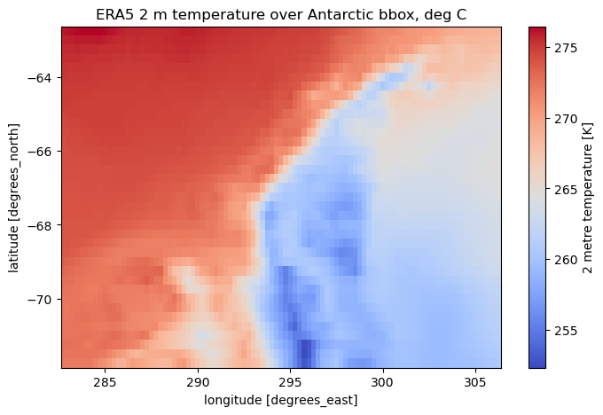
Example comparison
This is a quick exploratory example: compare coarse monthly-sampled ERA5 temperature between 1997 and 2016, then show the composite ice-mask boundaries for those years on top.
# ERA5 over the same lon/lat AOI
t2m = era5_ds["2m_temperature"].sel(
    longitude=slice(west % 360, east % 360),
    latitude=slice(north, south),
)

target_grid = ds.rio.set_spatial_dims(x_dim="x", y_dim="y").rio.write_crs("EPSG:3031")

with ProgressBar():
    # One timestep per month, then annual-ish mean
    t2m_1997 = t2m.sel(time=slice("1997-01-01", "1997-12-31")).isel(time=slice(0, None, 744)).mean("time")
    t2m_2016 = t2m.sel(time=slice("2016-01-01", "2016-12-31")).isel(time=slice(0, None, 744)).mean("time")

    t2m_change = t2m_2016 - t2m_1997

    t2m_change = (
        t2m_change
        .rio.set_spatial_dims(x_dim="longitude", y_dim="latitude")
        .rio.write_crs("EPSG:4326")
        .rio.reproject_match(target_grid)
        .compute()
    )

    mask_1997 = ds.icemask_composite.sel(time="1997-01-01", method="nearest").compute()
    mask_2016 = ds.icemask_composite.sel(time="2016-01-01", method="nearest").compute()

mask_footprint = (mask_1997 > 0) | (mask_2016 > 0)
mean_change = t2m_change.where(mask_footprint).mean().item()

fig, ax = plt.subplots(figsize=(8, 8))

t2m_change.plot(ax=ax, x="x", y="y", cmap="RdBu_r", center=0, robust=True)

mask_1997.plot.contour(ax=ax, x="x", y="y", levels=[0.5], colors="cyan")
mask_2016.plot.contour(ax=ax, x="x", y="y", levels=[0.5], colors="magenta")

ax.set_title(f"2016 - 1997 ERA5 monthly-sample 2 m temperature\nMean over ice-mask footprint: {mean_change:.2f}")
ax.set_aspect("equal")