Polar Hackathon - Polar Hackathon

This repository is a guided set of notebooks for discovering Antarctic datasets, converting them into cloud-native formats, combining them into analysis-ready collections, and using those collections in scientific workflows.

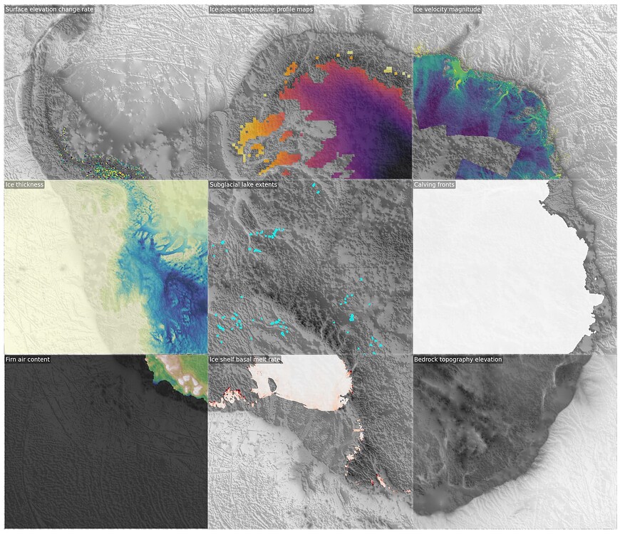
Repository Map¶

Folder	Purpose	Best starting point
`0_Introduction/`	Brief introduction to the hackathon, goals, EarthCODE context and agenda.	`0_Introduction/intro.ipynb`
`1_Datasets/`	Dataset catalogue and one access notebook per source product.	`1_Datasets/datasets_sumarry.ipynb`
`2_Datacube/`	Remote combined-cube access and examples for building a small cube.	`2_Datacube/1_remote_cube_access.ipynb`
`3_File_formats_and_metadata/`	Format conversion examples for Zarr, COG, GeoParquet, and the creation of STAC metadata.	`3_File_formats_and_metadata/0_intro.ipynb`
`4_Visualisation/`	Early visualisation experiments for interactive and static views.	`4_Visualisation/1_cog_visualisations.ipynb`
`5_Hackathon_Code/`	Your hackathon solution space. Put new work here unless a challenge asks otherwise.	Create your own notebook or package here.

Generated local data is expected in downloaded_data/, which is ignored by Git. The canonical copies of the prepared assets live in cloud object storage.

EarthCODE Context¶

The hackathon is supported by EarthCODE - the data is available on EarthCODE’s Open Science Catalog. The prepared assets demonstrate the path from domain-specific source products to cloud-native collections that can be inspected, combined, and cited.

The workflow to add data to these collections is to:

Start from a scientific product with its own native layout and metadata.
Convert or expose it as a cloud-native file format: Zarr for arrays, COG for rasters, GeoParquet for vectors and tables.
Add enough metadata for discovery, provenance, licensing, spatial extent, temporal extent, and variable interpretation.
Combine multiple products on a common analysis grid when that is scientifically defensible.

1. Datasets prepared for the hackathon.¶

Each of the datasets has an associated notebook, referenced in the access column that shows how the data can be accessed directly from object storage. More information about the datasets is available in the respective notebooks and the OSC pages. All notebooks reside in the 1_Datasets folder.

Dataset	Theme	Prepared format	CRS/grid	Time coverage	Licence	Links	Access notebook
AI4AIS Larsen C cube	Ice shelf combined variables	Zarr	EPSG:3031	Monthly from 2014 - 2021	CC-BY-NC-4.0	OSC	`ai4ais/access.ipynb`
ALBATROS tidal elevation	Altimetry tide elevation prediction	GeoParquet	Points in EPSG:4326, examples regrid to EPSG:3031	Example uses 2019 CryoSat-2 predictions	CC-BY-NC-4.0	OSC	`albatros/access.ipynb`
Ice shelf basal melt	Ice shelf melt rates	COG/GeoTIFF plus GeoParquet shelf time series	Antarctic polar stereographic, EPSG:3031	1997-2021	CC-BY-4.0	OSC	`basal_melt/access.ipynb`
BedMachine Antarctica	Bed, surface, thickness, mask	Zarr	Antarctic polar stereographic, EPSG:3031	Static product version	CC0-1.0	OSC	`bedrock_topography/access.ipynb`
Calving fronts	Time-evolving coastlines/fronts	GeoParquet	Vector geometries, examples reproject to EPSG:3031	Observation time series	CC-BY-4.0	OSC	`calving_fronts/access.ipynb`
CS+AO sea ice thickness	Southern Ocean sea ice	Zarr	Polar grid with lon/lat coordinates	CryoSat-2/SARAL period in source product	CC-BY-NC-4.0	OSC	`csao/access.ipynb`
Grounding lines	Antarctic grounding-line observations	GeoParquet	Vector geometries, examples reproject to EPSG:3031	1992-2014	CC0-1.0	OSC	`groundlines/access.ipynb`
Ice temperature profiles	Englacial temperature	Zarr, source NetCDF in format tutorials	Curvilinear source with lon/lat; examples reproject to EPSG:3031	data is from 2013-2014	CC-BY-4.0	OSC	`ice_temp/access.ipynb`
Ice velocity	Antarctic surface velocity	Zarr	Antarctic polar stereographic, EPSG:3031	Monthly, 2014-2021	CC-BY-NC-4.0	OSC	`ice_velocity/access.ipynb`
Surface elevation change	Grounded ice surface elevation	Zarr	Antarctic polar stereographic, EPSG:3031	1991-2021 5-year means	CC-BY-4.0	OSC	`sec/access.ipynb`
SOFRESH sea surface salinity	Southern Ocean salinity	Zarr	EASE-style Southern Ocean grid	2011-2022, 9-day maps	CC-BY-4.0	OSC	`sofresh/access.ipynb`
Subglacial lakes	Active lake boundaries	GeoParquet	Vector geometries, examples reproject to EPSG:3031	2010-2020 source analysis	CC-BY-4.0	OSC	`subglacial_lakes/access.ipynb`
Supraglacial lakes	Surface hydrology features	GeoParquet	Vector geometries	January 2017 maximum extent	CC-BY-4.0	OSC	`supraglacial_lakes/access.ipynb`

2. Datacube¶

As part of the initiative, and to facilitate easier analysis of and access to scientific Antarctica data, some of the presented datasets are combined into zarr stores, reprojected to a common 100x100m grid in the EPSG:3031 Polar projection.

You can see how to access the data from the access notebook
You can see how we combined the presented from the .combine notebook. Primarily we used nearest-neighbour interpolation. The goal was to provide single access to all the data in one place. You can use that notebook to combine the different raw datasets.
You can see how to carry larger-scale analysis efficiently in the large_area_processing notebook.

You can see a visualisation of the data in eodash: https://esa-earthcode.github.io/polar-science-cluster-dashboard/

You can also see examples of external data access and analysis alongside the with the cube data at Accessing External Datasets

3. File formats and metadata¶

We have also prepared some notebooks that show how we transformed the data from various file formats into the three cloud-optimised formats we have used and how we generated the associated metadata.

Dataset formats¶

All the original datasets have been converted to cloud-optimised formats. Primarily we used three formats

Format	Best for	Why it matters in object storage
Zarr	Multidimensional arrays such as time/depth/y/x cubes	Supports a flexible chunking scheme allows the indexing of data, optimised for analytics. Also, chunked reads let analysis load only the pieces it needs.
Cloud Optimized GeoTIFF (COG)	Single rasters or raster stacks exposed as files	Internal tiling and overviews enable efficient range reads and quicklooks.
GeoParquet	Vector geometries and tabular point data	Columnar storage, embedded geospatial metadata, and fast filtering.

For more information for each, checkout the notebooks or other resources like : https://guide.cloudnativegeo.org/

Metadata¶

For example datatype we also show how we genereated its associated metadata. Rich metadata ensures that the datasets are more accessible - https://esa-earthcode.github.io/documentation/Community and Best Practices/FAIR and Open Science Best Practices/Data.

All the metadata generated for the datasets and hosted on the Open Science Catalog is in STAC format. The SpatioTemporal Asset Catalog (STAC) specification was designed to establish a standard, unified language to talk about geospatial data, allowing it to be more easily searchable and queryable. For more information and a introduction to STAC, see https://esa-earthcode.github.io/tutorials/stac-and-data-access/ .