This notebook is a runnable remote-access demo for the published ESA Antarctica land-ice GeoZarr stores. It opens full-resolution group 0; use groups 1 through 4 for progressively coarser multiscale levels.
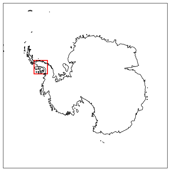
The example uses a small Palmer Land / George VI Ice Shelf ROI. Change ROI_CENTER_XY_M or ROI_HALF_WIDTH_CELLS to explore another area. Remote reads still happen at the Zarr chunk level, so keep the ROI inside one chunk-sized area for quick laptop runs.
Setup
Set CUBE_LEVEL to "0" for full resolution or to "1" through "4" for a coarser common GeoZarr level. The five published stores can then be opened as one lazy dataset with open_mfdataset. Because SEC, velocity, and the composite ice mask use a time dimension, xarray aligns them on the outer union of their timestamps; select dates explicitly when using those variables.
import numpy as np
import warnings
import xarray as xr
from dask.array.core import PerformanceWarning
from dask.diagnostics import ProgressBar
from matplotlib.colors import BoundaryNorm, ListedColormap
from matplotlib.patches import Rectangle

import matplotlib.pyplot as plt
import cartopy.crs as ccrs

warnings.filterwarnings("ignore", message="In a future version of xarray the default value for join.*", category=FutureWarning)
warnings.filterwarnings("ignore", message="Increasing number of chunks.*", category=PerformanceWarning)

# Approximate EPSG:3031 location for Palmer Land / George VI Ice Shelf.
ROI_CENTER_XY_M = (-2_000_000.0, 800_000.0)
ROI_HALF_WIDTH_CELLS = 3000
VELOCITY_VECTOR_STRIDE = 90
VELOCITY_TIME_TARGET = "2021-12-01"
SEC_TIME_TARGET = "2020-01-01"
TEMPERATURE_DEPTH_TARGET_M = 1000

antarctic_crs = ccrs.SouthPolarStereo(
    central_longitude=0,
    true_scale_latitude=-71,
)
# Convert ROI center from meters to the appropriate scale and calculate half-width
cx, cy = ROI_CENTER_XY_M
half = ROI_HALF_WIDTH_CELLS * 100
fig, ax = plt.subplots(figsize=(7, 7), subplot_kw={"projection": ccrs.SouthPolarStereo()})
ax.set_extent([-180, 180, -90, -58], crs=ccrs.PlateCarree())
ax.coastlines()
ax.add_patch(Rectangle((cx - half, cy - half), 2 * half, 2 * half, fill=False, edgecolor="red", linewidth=2, transform=ax.projection))
plt.show()
CUBE_LEVEL = "0"
cube_paths = [
    "https://s3.waw4-1.cloudferro.com/EarthCODE/OSCAssets/antarctica_cube/land-ice/ice-temp-cube.zarr",
    "https://s3.waw4-1.cloudferro.com/EarthCODE/OSCAssets/antarctica_cube/land-ice/sec.zarr",
    "https://s3.waw4-1.cloudferro.com/EarthCODE/OSCAssets/antarctica_cube/land-ice/antarctica-combined.zarr",
    "https://s3.waw4-1.cloudferro.com/EarthCODE/OSCAssets/antarctica_cube/land-ice/icemask_composite.zarr",
    "https://s3.waw4-1.cloudferro.com/EarthCODE/OSCAssets/antarctica_cube/land-ice/ice_velocity.zarr",
]

ds = xr.open_mfdataset(cube_paths, engine="zarr", group=CUBE_LEVEL, chunks={}, compat="no_conflicts", join="outer")

ds
Select A Small Region Of Interest
The land/ice cubes share the same y, x grid. The helper below snaps the
requested EPSG:3031 point to the nearest cube cell and builds one integer ROI
slice that is reused for every cube.
x_index = int(np.abs(ds["x"].values - ROI_CENTER_XY_M[0]).argmin())
y_index = int(np.abs(ds["y"].values - ROI_CENTER_XY_M[1]).argmin())
x_slice = slice(x_index - ROI_HALF_WIDTH_CELLS, x_index + ROI_HALF_WIDTH_CELLS + 1)
y_slice = slice(y_index - ROI_HALF_WIDTH_CELLS, y_index + ROI_HALF_WIDTH_CELLS + 1)

small = ds.isel(x=x_slice, y=y_slice).chunk({"x": -1, "y": -1})

small
Plot 1: Bedrock Topography And Thickness Above Flotation
This reproduces the bedrock-topography use case on the remote cube. It combines
BedMachine-style bed, thickness, and mask variables to estimate thickness
above flotation for grounded marine ice. Low values identify ice that is closer
to flotation.
rho_ice = 917.0
rho_water = 1027.0

bed = small["bed"]
thickness = small["thickness"]
mask = small["mask"]

flotation_thickness = xr.where(bed < 0, -(rho_water / rho_ice) * bed, 0)
taf = (thickness - flotation_thickness).where((mask == 2) & (bed < 0)).clip(0, 500)

with ProgressBar():
    taf = taf.compute()

fig, ax = plt.subplots(figsize=(8, 8), subplot_kw={"projection": antarctic_crs})
taf.plot(ax=ax, cmap="viridis_r", vmin=0, vmax=500, transform=antarctic_crs)
ax.coastlines()
Plot 2: Ice-Shelf Basal Melt Rate
The basal-melt workflow is available as a raster layer in the combined cube. This plot shows the melt-rate field for the same ROI. The original shelf-name polygon time series is not part of these raster cubes, but the gridded melt-rate field is ready for spatial overlay and small-area statistics.
basal_melt = small["ice_shelf_basal_melt_rate"]

with ProgressBar():
    basal_melt = basal_melt.compute()

fig, ax = plt.subplots(figsize=(8, 8), subplot_kw={"projection": antarctic_crs})
basal_melt.plot(ax=ax, cmap="RdBu_r", robust=True, transform=antarctic_crs)
ax.coastlines()
Plot 3: Surface Elevation Change
The SEC cube stores gridded surface-elevation-change rates by time period. This example takes the latest period, masks to grounded ice, converts metres to millimetres, and plots the spatial fingerprint of elevation gain or loss.
sec_rate = small["sec"].sel(time=SEC_TIME_TARGET) * 1000
sec_grounded = small["surface_type"] == 2
sec_rate = sec_rate.where(sec_grounded)

with ProgressBar():
    sec_rate = sec_rate.compute()

fig, ax = plt.subplots(figsize=(8, 8), subplot_kw={"projection": antarctic_crs})
sec_rate.plot(ax=ax, cmap="RdBu_r", vmin=-500, vmax=500, transform=antarctic_crs)
ax.coastlines()
Plot 4: Englacial Temperature At A Selected Depth
The source temperature notebook reprojected a non-regular source product. In the
remote cube, ice temperature is already on the shared EPSG:3031 grid. This plot
selects the depth nearest TEMPERATURE_DEPTH_TARGET_M.
ice_temp_c = small["Tice"].sel(depth=TEMPERATURE_DEPTH_TARGET_M, method="nearest")

with ProgressBar():
    ice_temp_c = ice_temp_c.compute()

fig, ax = plt.subplots(figsize=(8, 8), subplot_kw={"projection": antarctic_crs})
ice_temp_c.plot(ax=ax, cmap="coolwarm", robust=True, transform=antarctic_crs)
ax.coastlines()
Plot 5: Composite Ice-Mask Change
The composite ice-mask GeoZarr contains annual Antarctic ice masks from 1997 to 2021. This example compares the first and last available masks in the ROI, highlighting where the binary mask changed through time.
ice_mask = small["icemask_composite"]

with ProgressBar():
    available_times = ice_mask.notnull().any(("x", "y")).compute()

ice_mask = ice_mask.isel(time=available_times.values)
ice_mask_change = ice_mask.isel(time=-1) - ice_mask.isel(time=0)

with ProgressBar():
    ice_mask_change = ice_mask_change.compute()

fig, ax = plt.subplots(figsize=(8, 8), subplot_kw={"projection": antarctic_crs})
ice_mask_change.plot(ax=ax, cmap="RdBu_r", vmin=-1, vmax=1, transform=antarctic_crs)
ax.coastlines()
Plot 6: Grounding Lines And Lake Masks
The groundline, subglacial-lake, and supraglacial-lake workflows are available
as raster masks in the combined cube. This plot combines them into one class-code
image for a compact overview: 1 marks supraglacial lakes/channels, 2 marks
subglacial lakes, and 4 marks grounding-line pixels. Sums indicate overlap.
mask_code = (
    (small["supra_glacial_lakes_mask"] > 0).astype("uint8")
    + 2 * (small["subglacial_lakes_extents_mask"] > 0).astype("uint8")
    + 4 * (small["groundlines_mask"] > 0).astype("uint8")
)

with ProgressBar():
    mask_code = mask_code.compute()

mask_cmap = ListedColormap(["white", "#4f9cf9", "#8e44ad", "#1f9d55", "#111111", "#f59e0b", "#d946ef", "#ef4444"])
mask_norm = BoundaryNorm(np.arange(-0.5, 8.5), mask_cmap.N)

# mask_code.plot(cmap=mask_cmap, norm=mask_norm, cbar_kwargs={"ticks": range(8)})

fig, ax = plt.subplots(figsize=(8, 8), subplot_kw={"projection": antarctic_crs})
mask_code.plot(ax=ax, cmap=mask_cmap, norm=mask_norm, cbar_kwargs={"ticks": range(8)}, transform=antarctic_crs)
ax.coastlines()
Plot 7: Ice Velocity Vectors Over Basal Melt
The velocity cube provides easting, northing, and magnitude variables on the same remote grid. This section samples the latest time step coarsely for arrows and plots those vectors over the basal-melt raster computed earlier.
stride = VELOCITY_VECTOR_STRIDE

background = small["ice_shelf_basal_melt_rate"]
u = small["land_ice_surface_easting_velocity"].sel(time=VELOCITY_TIME_TARGET).isel(y=slice(None, None, stride), x=slice(None, None, stride))
v = small["land_ice_surface_northing_velocity"].sel(time=VELOCITY_TIME_TARGET).isel(y=slice(None, None, stride), x=slice(None, None, stride))
with ProgressBar():
    background = background.compute()
    u = u.compute()
    v = v.compute()

X, Y = np.meshgrid(u["x"].values, u["y"].values)

fig, ax = plt.subplots(figsize=(8, 8), subplot_kw={"projection": antarctic_crs})

background.plot(ax=ax, cmap="RdBu_r", robust=True, transform=antarctic_crs)
ax.quiver(X, Y, u.values, v.values, width=0.0025, transform=antarctic_crs)
ax.coastlines()

plt.show()