Explore Data · Explore Data · Explore Data · Explore Data
This notebook opens the four online stores of the ESA Mediterranean Sea Datacube and plots selected variables. Group 0 provides full resolution; groups 1 and 2 provide coarser spatial summaries.
The example uses a small Alboran Sea ROI. Change ROI_CENTER_LON_LAT or ROI_HALF_WIDTH_CELLS to explore another area. Reads happen at the Zarr chunk level, so a small selection may still read a larger stored chunk.
Setup
Set CUBE_LEVEL to "0" for full resolution, "1" for 1/6°, or "2" for 1/3°. Each cube is opened with xr.open_zarr when it is needed below. The examples use June 2019.
import numpy as np
import xarray as xr
from dask.diagnostics import ProgressBar
from matplotlib.patches import Rectangle
import matplotlib.pyplot as plt

CUBE_LEVEL = "0"
ROI_CENTER_LON_LAT = (-2.5, 36.0)
ROI_HALF_WIDTH_CELLS = 100
VELOCITY_VECTOR_STRIDE = 6
DAILY_TIME_TARGET = "2019-06-01"
MONTHLY_TIME_TARGET = "2019-06-01"
HOURLY_TIME_TARGET = "2019-06-01T12:00:00"
BIOPHYSICS_DEPTH_TARGET_M = 19.0
Open the Daily Surface Cube
Start with the daily surface cube for the region map, salinity, density, and sea-level examples.
daily_surface_cube = xr.open_zarr(
    "https://s3.waw4-1.cloudferro.com/EarthCODE/OSCAssets/med_cubes/ocean-med-daily-surface-cube.zarr",
    group=CUBE_LEVEL, chunks={}, consolidated=True, decode_coords="all",
)
daily_surface_cubeSelect A Small Region Of Interest
Select a region from the daily surface cube. The code snaps the requested point to the nearest grid cell and clips the slices at the cube edges. All four stores share the same horizontal grid, so the later examples reuse these slices.
x_index = int(np.abs(daily_surface_cube.lon.values - ROI_CENTER_LON_LAT[0]).argmin())
y_index = int(np.abs(daily_surface_cube.lat.values - ROI_CENTER_LON_LAT[1]).argmin())
x_slice = slice(max(0, x_index - ROI_HALF_WIDTH_CELLS),
                min(daily_surface_cube.sizes["lon"], x_index + ROI_HALF_WIDTH_CELLS + 1))
y_slice = slice(max(0, y_index - ROI_HALF_WIDTH_CELLS),
                min(daily_surface_cube.sizes["lat"], y_index + ROI_HALF_WIDTH_CELLS + 1))
surface_region = daily_surface_cube.isel(lon=x_slice, lat=y_slice)
surface_regionregion = surface_region
fig, ax = plt.subplots(figsize=(10, 4))
daily_surface_cube.water_mask.plot(ax=ax, cmap="Blues", add_colorbar=False)
ax.add_patch(Rectangle(
(float(region.lon.min()), float(region.lat.min())),
float(region.lon.max() - region.lon.min()),
float(region.lat.max() - region.lat.min()),
fill=False, edgecolor="red", linewidth=2,
))
ax.set_title("Alboran Sea ROI on the Mediterranean water retention mask")
plt.show()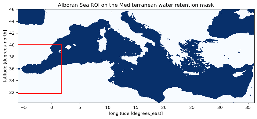
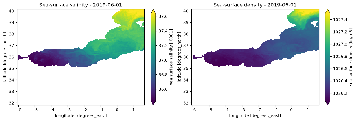
Plot 1: Sea-Surface Salinity And Density
with ProgressBar():
    surface = surface_region[["sos", "dos"]].sel(time=DAILY_TIME_TARGET).compute()

fig, axes = plt.subplots(1, 2, figsize=(12, 4), constrained_layout=True)
for ax, name, title in zip(axes, ["sos", "dos"], ["Sea-surface salinity", "Sea-surface density"]):
    surface[name].plot(ax=ax, cmap="viridis", robust=True)
    ax.set_title(f"{title} - {DAILY_TIME_TARGET}")
plt.show()
[########################################] | 100% Completed | 202.01 ms
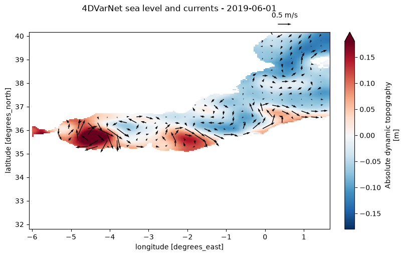
Plot 2: Sea Level And Geostrophic Currents
with ProgressBar():
    sea_level = surface_region[[
        "adt_4dvarnet", "ugos_4dvarnet", "vgos_4dvarnet"
    ]].sel(time=DAILY_TIME_TARGET).compute()

fig, ax = plt.subplots(figsize=(8, 5), constrained_layout=True)
sea_level.adt_4dvarnet.plot(ax=ax, cmap="RdBu_r", robust=True)
vectors = sea_level.isel(lat=slice(None, None, VELOCITY_VECTOR_STRIDE),
                         lon=slice(None, None, VELOCITY_VECTOR_STRIDE))
q = ax.quiver(vectors.lon, vectors.lat, vectors.ugos_4dvarnet, vectors.vgos_4dvarnet)
ax.quiverkey(q, 0.85, 1.04, 0.5, "0.5 m/s")
ax.set_title(f"4DVarNet sea level and currents - {DAILY_TIME_TARGET}", pad=30)
plt.show()
[########################################] | 100% Completed | 201.62 ms
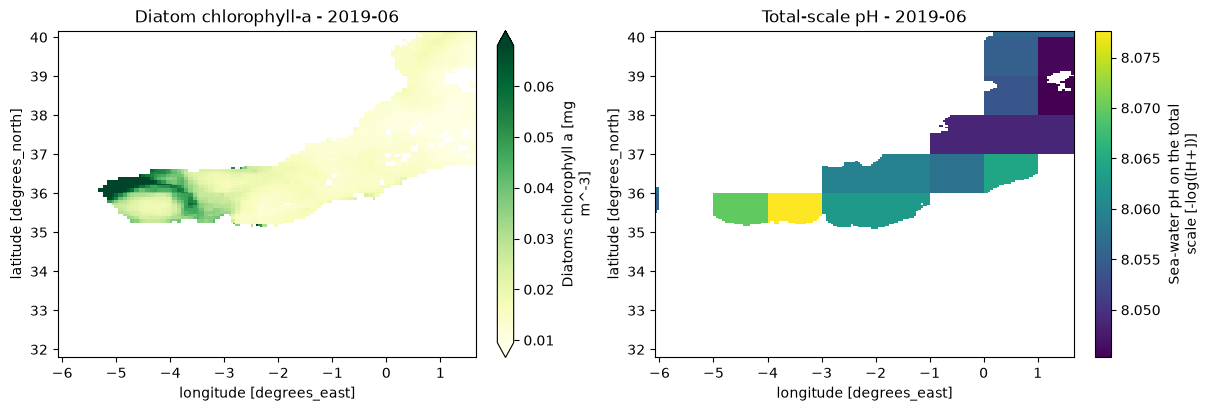
Plot 3: Phytoplankton And Carbonate Chemistry
monthly_cube = xr.open_zarr(
    "https://s3.waw4-1.cloudferro.com/EarthCODE/OSCAssets/med_cubes/ocean-med-monthly-cube.zarr",
    group=CUBE_LEVEL, chunks={}, consolidated=True, decode_coords="all",
)

with ProgressBar():
    monthly = (monthly_cube[["DIATO", "ph_total"]]
               .isel(lon=x_slice, lat=y_slice)
               .sel(time=MONTHLY_TIME_TARGET).compute())

fig, axes = plt.subplots(1, 2, figsize=(12, 4), constrained_layout=True)
monthly.DIATO.plot(ax=axes[0], cmap="YlGn", robust=True)
monthly.ph_total.plot(ax=axes[1], cmap="viridis", robust=True)
axes[0].set_title(f"Diatom chlorophyll-a - {MONTHLY_TIME_TARGET[:7]}")
axes[1].set_title(f"Total-scale pH - {MONTHLY_TIME_TARGET[:7]}")
plt.show()
[########################################] | 100% Completed | 403.09 ms
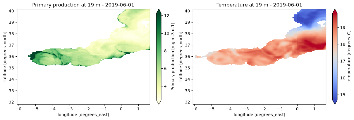
Plot 4: Primary Production And Temperature At A Selected Depth
biophysics_cube = xr.open_zarr(
    "https://s3.waw4-1.cloudferro.com/EarthCODE/OSCAssets/med_cubes/ocean-med-biophysics.zarr",
    group=CUBE_LEVEL, chunks={}, consolidated=True, decode_coords="all",
)

with ProgressBar():
    biophysics = (biophysics_cube[["PP", "to"]].isel(lon=x_slice, lat=y_slice)
                  .sel(time=DAILY_TIME_TARGET)
                  .sel(depth=BIOPHYSICS_DEPTH_TARGET_M).compute())
selected_depth = float(biophysics.depth)

fig, axes = plt.subplots(1, 2, figsize=(12, 4), constrained_layout=True)
biophysics.PP.plot(ax=axes[0], cmap="YlGn", robust=True, cbar_kwargs={"label": "Primary production [mg m-3 d-1]"})
biophysics["to"].plot(ax=axes[1], cmap="coolwarm", robust=True)
axes[0].set_title(f"Primary production at {selected_depth:g} m - {DAILY_TIME_TARGET}")
axes[1].set_title(f"Temperature at {selected_depth:g} m - {DAILY_TIME_TARGET}")
plt.show()
[########################################] | 100% Completed | 1.21 ss
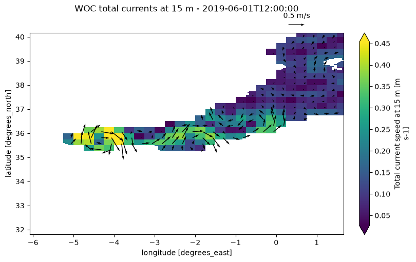
Plot 5: Hourly Total Currents At 15 m
hourly_cube = xr.open_zarr(
    "https://s3.waw4-1.cloudferro.com/EarthCODE/OSCAssets/med_cubes/hourly_cube.zarr",
    group=CUBE_LEVEL, chunks={}, consolidated=True, decode_coords="all",
)

with ProgressBar():
    hourly = (hourly_cube[["ut_woc", "vt_woc"]].isel(lon=x_slice, lat=y_slice)
              .sel(time=HOURLY_TIME_TARGET, depth=15.0).compute())

speed = np.hypot(hourly.ut_woc, hourly.vt_woc).rename("current_speed")
speed.attrs.update(long_name="Total current speed at 15 m", units="m s-1")
fig, ax = plt.subplots(figsize=(8, 5), constrained_layout=True)
speed.plot(ax=ax, cmap="viridis", robust=True)
vectors = hourly.isel(lat=slice(None, None, VELOCITY_VECTOR_STRIDE),
                      lon=slice(None, None, VELOCITY_VECTOR_STRIDE))
q = ax.quiver(vectors.lon, vectors.lat, vectors.ut_woc, vectors.vt_woc)
ax.quiverkey(q, 0.85, 1.04, 0.5, "0.5 m/s")
ax.set_title(f"WOC total currents at 15 m - {HOURLY_TIME_TARGET}", pad=30)
plt.show()
[########################################] | 100% Completed | 201.39 ms
Inspect Variable Metadata
Check the units, provenance, and processing metadata before combining products. The overview explains source naming, coverage gaps, and aggregation.
biophysics_cube["PP"].attrs{'processing_steps': {'regrid_func': 'regrid_kdtree_pyresample',
'roi_m': 4000,
'epsilon': 0},
'standard_name': 'net_primary_production_of_biomass_expressed_as_carbon_per_unit_volume_in_sea_water',
'long_name': 'Primary Production field estimated from chlorophyll and temperature 3D fields [spatial resolution = 1/24 deg]',
'description': 'Primary Production field estimated from chlorophyll and temperature 3D fields [spatial resolution = 1/24 deg]',
'units': 'mg m-3 d-1',
'source': 'https://esa-earthcode.github.io/open-science-catalog-metadata/products/4dmed-3d-prim-prod-150/collection',
'reference': 'https://4dmed.artov.ismar.cnr.it/thredds/catalog/4dmed/catalog_PP.html',
'original_spatial_resolution': [0.04166666478007059, 0.0416666683530934],
'original_temporal_resolution': '1 days 00:00:00',
'file_type': 'area',
'is_mask': False,
'data_meaning': 'continuous',
'valid_range': [3.0095383730446977e-25, 923.970458984375],
'visualization_range': [4.001231412887574, 14.316554222106928],
'aggregation_method': 'mean'}Close The Datasets
daily_surface_cube.close()
monthly_cube.close()
biophysics_cube.close()
hourly_cube.close()