Time Series at Every Depth - Ocean Hackathon

This notebook shows how to setup a dask cluster on the platofrm or locally to do longer-running jobs. It uses a temperature across time and depth plot as an example.

import dask.array as da
import dask.distributed
import warnings
import numpy as np
import xarray as xr
from dask.array.core import PerformanceWarning
# from dask_gateway import Gateway

warnings.filterwarnings("ignore", message="In a future version of xarray the default value for join.*", category=FutureWarning)
warnings.filterwarnings("ignore", message="Increasing number of chunks.*", category=PerformanceWarning)

## run this line if you get a file system not found error!
# import os
# os.chdir("/tmp")
# print("cwd:", os.getcwd())

Dask Cluster Setup¶

Use the Dask Gateway cells on the cloud workspace. For local runs, skip the Gateway cells and run the local alternative cell instead.

# Local alternative: run this cell instead of the Dask Gateway cells below.
cluster = dask.distributed.LocalCluster(
    n_workers=2,
    threads_per_worker=2,
    memory_limit="4GB",
)
client = dask.distributed.Client(cluster)
client

Cloud Workspace¶

gateway = Gateway()
cluster_options = gateway.cluster_options()
cluster_options

cluster = gateway.new_cluster(cluster_options=cluster_options)
cluster.scale(2)
cluster

client = cluster.get_client()
client

import matplotlib.pyplot as plt

Open the Biophysics Dataset¶

Open level 0 at full spatial resolution. The data remain lazy until we load the selected time series below.

INPUT_PATH = "https://s3.waw4-1.cloudferro.com/EarthCODE/OSCAssets/med_cubes/ocean-med-biophysics.zarr"

ds = xr.open_zarr(INPUT_PATH, group="0", chunks={}, consolidated=True, decode_coords="all")

Select a Location and Year¶

to is sea-water temperature. Select the nearest grid point to 2.5°W, 36°N and keep every depth for 2019. Change the longitude, latitude, or dates to explore another location or period.

The selection stays lazy. Plotting below computes it using the active Dask client.

temperature = (
    ds["to"]
    .sel(lon=-2.5, lat=36.0, method="nearest")
    .sel(time=slice("2019-01-01", "2019-12-31"))
)
temperature

Plot Temperature Through Time and Depth¶

Each row shows the temperature time series at a depth, with deeper water lower on the plot. Colour shows temperature, making seasonal warming and cooling easy to compare across depths.

temperature.plot(
    x="time", y="depth", yincrease=False,
    cmap="RdYlBu_r", figsize=(12, 5),
)
plt.title("Sea-water temperature in the Alboran Sea")
plt.xlabel("Date")
plt.ylabel("Depth (m)")
plt.show()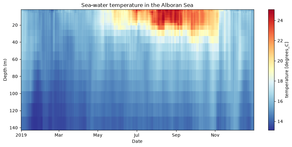

ds.close()
client.close()
cluster.close()