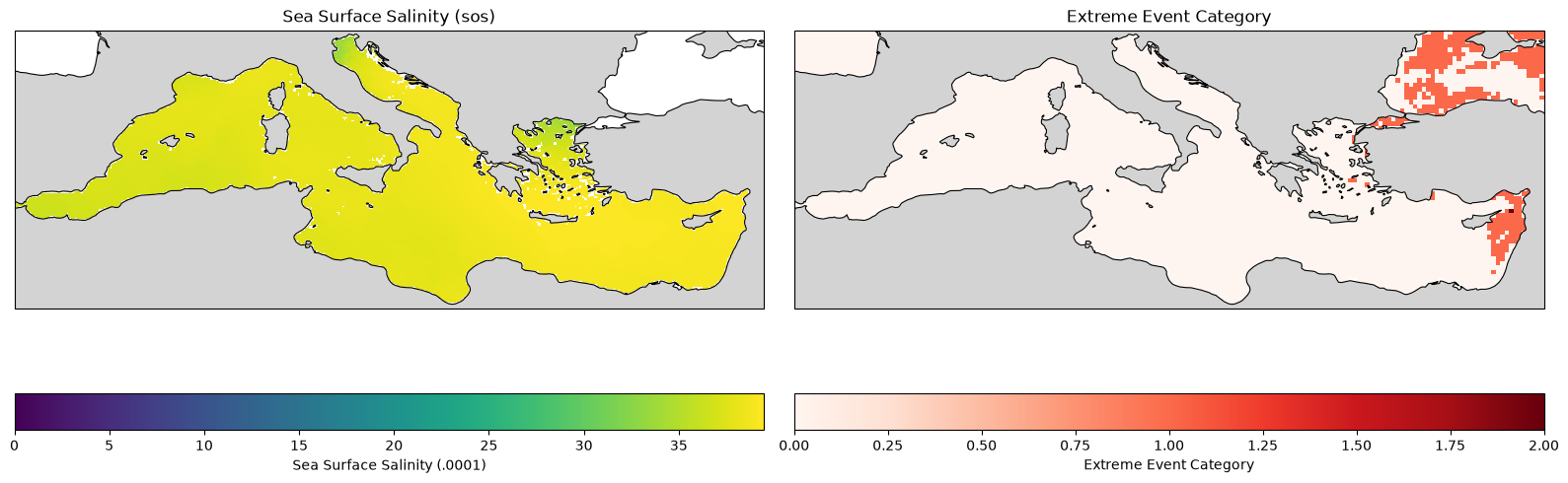
This notebooks shows how to regrid and combine two datasets from different sources and with different resolutions. The first one is the 4DMED-SEA sea-surface salinity and the second one Careheat.
The code specifies a day, resamples the datasets to a 1/12° grid, applies the WorldCover water retention mask, saves the results as Zarr v3, and plots the result.
The datacubes were created following a similar procedure. The overview describes the original cube workflows.
from pathlib import Path

import geopandas as gpd
import numpy as np
import rioxarray
import xarray as xr
import matplotlib.pyplot as plt
from dask.diagnostics import ProgressBar
from rasterio.enums import Resampling
from rioxarray.merge import merge_arrays


FINAL_CUBE = "alboran_daily_demo_cube.zarr"
1. Open the Source Dataset
Open the 4DMED-SEA salinity dataset. The data remain lazy until the selected region is written below.
INPUT_PATH1 = "https://s3.waw4-1.cloudferro.com/EarthCODE/OSCAssets/ocean_datasets/sssd.zarr"
INPUT_PATH2 = "https://s3.waw4-1.cloudferro.com/EarthCODE/OSCAssets/ocean_datasets/careheat_mhw_2d.zarr"


source_dataset1 = xr.open_zarr(
    INPUT_PATH1, chunks={}, decode_coords="all",
)
source_dataset2 = xr.open_zarr(
    INPUT_PATH2, chunks={}, decode_coords="all",
)
2. Select a date and resample both datasets
Create the new grid, select surface salinity (depth=0) and the careheat category data for the same day, for the whole of the Med and copy the nearest source value to each target cell.
# 1. Define bounding box for the Mediterranean Sea
LON_MIN, LON_MAX = -6.0, 37.0   # From the Strait of Gibraltar to the Levantine coast
LAT_MIN, LAT_MAX = 30.0, 46.0   # From the North African coast to the northern Adriatic
TARGET_RESOLUTION_DEG = 1 / 12
TIME_TARGET = "2019-06-01"

# 2. Calculate the number of cells for longitude and latitude separately
n_cells_lon = int(round((LON_MAX - LON_MIN) / TARGET_RESOLUTION_DEG))
n_cells_lat = int(round((LAT_MAX - LAT_MIN) / TARGET_RESOLUTION_DEG))

# 3. Create 1D coordinate arrays (cell centers)
target_lon = LON_MIN + (np.arange(n_cells_lon) + 0.5) * TARGET_RESOLUTION_DEG
target_lat = LAT_MIN + (np.arange(n_cells_lat) + 0.5) * TARGET_RESOLUTION_DEG
source1 = source_dataset1[["sos"]].sel(
time=slice(TIME_TARGET, TIME_TARGET), depth=0, drop=True,
lon=slice(LON_MIN - 0.25, LON_MAX + 0.25),
lat=slice(LAT_MIN - 0.25, LAT_MAX + 0.25),
)
source2 = source_dataset2[["category"]].sel(
time=slice(TIME_TARGET, TIME_TARGET), drop=True,
lon=slice(LON_MIN - 0.25, LON_MAX + 0.25),
lat=slice(LAT_MIN - 0.25, LAT_MAX + 0.25),
)sss = source1.interp(lon=target_lon, lat=target_lat, method="nearest")
caheat_cat = source2.interp(lon=target_lon, lat=target_lat, method="nearest")
# align the time coordinates
sss['time'] = caheat_cat['time']
cube = xr.merge([sss, caheat_cat])
cube = cube.rio.write_crs("EPSG:4326").rio.set_spatial_dims(x_dim="lon", y_dim="lat")
cubefig, ax = plt.subplots(nrows=1, ncols=2, figsize=(10,5))
cube.sos.isel(time=0).plot(ax=ax[0])
cube.category.isel(time=0).plot(ax=ax[1])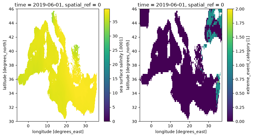
3. Apply the WorldCover Water Retention Mask
Read the roughly 320 m overviews of the ESA WorldCover 2021 tiles covering this region. Classes 0 (unmapped) and 80 (permanent water) are retained. Minimum resampling excludes a target cell if it contains mapped land; areas outside the mosaic remain retained. Unmapped areas are not confirmed water.
Apply the spatial mask to salinity across time and keep water_mask in the output (1 retained, 0 excluded).
left, bottom, right, top = cube.rio.bounds()
WC_BASE = "https://esa-worldcover.s3.eu-central-1.amazonaws.com"
tiles = gpd.read_file(f"{WC_BASE}/v100/2020/esa_worldcover_2020_grid.geojson").cx[left:right, bottom:top]
wc = merge_arrays([
    rioxarray.open_rasterio(
        f"{WC_BASE}/v200/2021/map/ESA_WorldCover_10m_2021_v200_{tile}_Map.tif",
        overview_level=4,
    )
    for tile in sorted(tiles.ll_tile)
], nodata=0).squeeze("band", drop=True)

water = wc.isin([0, 80]).astype("uint8").rio.write_nodata(255)
water_mask = water.rio.reproject_match(cube, resampling=Resampling.min, nodata=255)
water_mask = water_mask.where(water_mask != 255, 1)
water_mask = water_mask.rename({"x": "lon", "y": "lat"}).rename("water_mask")
cube["sos"] = cube.sos.where(water_mask == 1)
cube["water_mask"] = water_mask
cube.sos.isel(time=0).plot()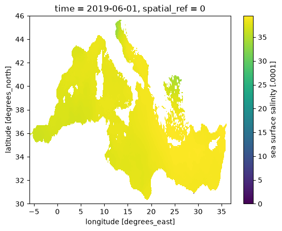
4. Save the Local Cube
Record the coordinate system, grid spacing, and source, then write the masked salinity and water_mask to downloaded_data/alboran_daily_demo_cube.zarr.
mode="w-" keeps an existing result from being overwritten. Choose a new output filename to run the write again.
cube.attrs = {
    "title": "Alboran Sea salinity demonstration cube",
    "crs": "EPSG:4326",
    "target_resolution_degrees": TARGET_RESOLUTION_DEG,
    "source_store1": INPUT_PATH1,
    "source_store2": INPUT_PATH2,
    "interpolation_method": "nearest",
}

# Clear the source storage settings before writing the new grid.
for name in cube.variables:
    cube[name].encoding = {}
for name in cube.data_vars:
    cube[name].attrs["grid_mapping"] = "spatial_ref"

with ProgressBar():
    cube.chunk({"time": 1, "lat": -1, "lon": -1}).to_zarr(
        FINAL_CUBE, mode="w", consolidated=True, zarr_format=3,
    )
[################ ] | 41% Completed | 100.65 ms/home/krasen/hackathon_websites/ocean_hackathon/.pixi/envs/default/lib/python3.13/site-packages/zarr/api/asynchronous.py:231: ZarrUserWarning: Consolidated metadata is currently not part in the Zarr format 3 specification. It may not be supported by other zarr implementations and may change in the future.
warnings.warn(
[########################################] | 100% Completed | 1.51 sms
5. Open and Plot the Result
Read the local cube and plot sea-surface salinity for the selected day.
import matplotlib.pyplot as plt
import cartopy.crs as ccrs
import cartopy.feature as cfeature


combined_ds = xr.open_zarr(FINAL_CUBE, consolidated=True, decode_coords="all")
ds_plot = combined_ds.isel(time=0)

fig, axes = plt.subplots(
    nrows=1, ncols=2,
    figsize=(16, 6),
    subplot_kw={'projection': ccrs.PlateCarree()}
)


# ---------------------------------------------------------
# Plot 1: Sea Surface Salinity (sos)
# ---------------------------------------------------------
ds_plot['sos'].plot(
    ax=axes[0],
    transform=ccrs.PlateCarree(),
    cmap='viridis',
    cbar_kwargs={'label': 'Sea Surface Salinity (.0001)', 'orientation': 'horizontal'}
)
axes[0].set_title('Sea Surface Salinity (sos)')

# ---------------------------------------------------------
# Plot 2: Extreme Event Category (category)
# ---------------------------------------------------------
ds_plot['category'].plot(
    ax=axes[1],
    transform=ccrs.PlateCarree(),
    cmap='Reds', # A sequential colormap is usually good for categorical/extreme data
    cbar_kwargs={'label': 'Extreme Event Category', 'orientation': 'horizontal'}
)
axes[1].set_title('Extreme Event Category')

for ax in axes:
    # Add land mask (zorder=1 to ensure it draws on top of any NaN ocean artifacts, or underneath data)
    ax.add_feature(cfeature.LAND, facecolor='lightgray', zorder=1)

    # Add coastlines
    ax.coastlines(resolution='50m', color='black', linewidth=0.8, zorder=2)

    # Restrict the plot extent to your Mediterranean bounds
    # Format: [lon_min, lon_max, lat_min, lat_max]
    ax.set_extent([-6.0, 37.0, 30.0, 46.0], crs=ccrs.PlateCarree())

plt.tight_layout()
plt.show()