The EDC (Euro Data Cube) workspace provides Dask Gateway for scalable analysis of collections that are larger than memory. This notebook starts with a local Dask client and uses the 4DMED-SEA sea-surface salinity collection as an ocean example.
The same workflow can then be moved to the Dask Gateway provided by EDC.
import xarray as xr
from dask.distributed import Client
What Is Dask?
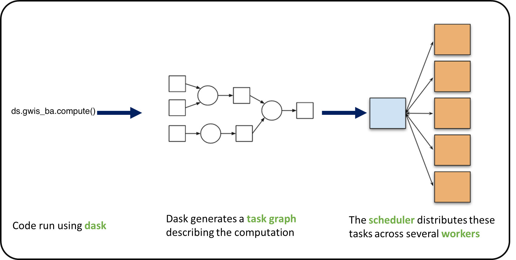
Dask extends familiar Python array and dataframe libraries with lazy, parallel execution. Xarray can represent a large remote array as many smaller chunks and build a task graph before any values are loaded. Computation begins only when an operation such as compute(), load(), or plotting requests a result.
This separation between describing and executing a workflow lets you inspect the planned work, select only the required data, and scale from a laptop to a distributed cluster with few code changes.
A generic example of task graphs and worker scheduling:
Start a Local Client
A local client is sufficient for learning, developing a workflow, and testing small selections. The client also provides a Dask Dashboard link for inspecting tasks, memory, and worker activity.
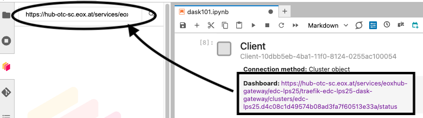
client = Client()
clientOptional Dask Gateway
EDC provides Dask Gateway for creating distributed clusters. Available cluster profiles and resource limits can be inspected with Gateway().cluster_options(). Uncomment this cell in EDC and keep it commented when working locally.
Please don’t run this during the main sessions. If many people start clusters together during the workshop, the auto-scaler will take quite a bit of time to create new workers.
# from dask_gateway import Gateway
# gateway = Gateway()
# cluster = gateway.new_cluster()
# cluster.scale(2)
# client.close()
# client = cluster.get_client()
Open an Ocean Collection Lazily
The following Zarr store contains Mediterranean sea-surface salinity and density fields. Passing chunks={} keeps the arrays lazy so opening the collection reads metadata rather than loading the full dataset.
from pystac_client import Client as STACClient

catalog = STACClient.open("https://eoapi.workspace.earthcode.eox.at/stac/")
item = next(catalog.search(collections=["4dmed-2d-sss"]).items())
itemitem.assets["data"].hrefdataset = xr.open_zarr(item.assets["data"].href, chunks={})
datasetBuild a Small Task Graph
Select one date and the surface layer, then coarsen the spatial grid. These operations construct a task graph without immediately downloading all source chunks.
salinity = dataset["sos"].sel(
    time="2020-06-15",
    depth=0,
    method="nearest",
    drop=True,
)

plot_data = salinity.coarsen(
    lat=4,
    lon=4,
    boundary="trim",
).mean()

plot_data.dataplot_data.data.visualize(optimize_graph=True)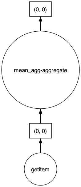
Compute and Plot
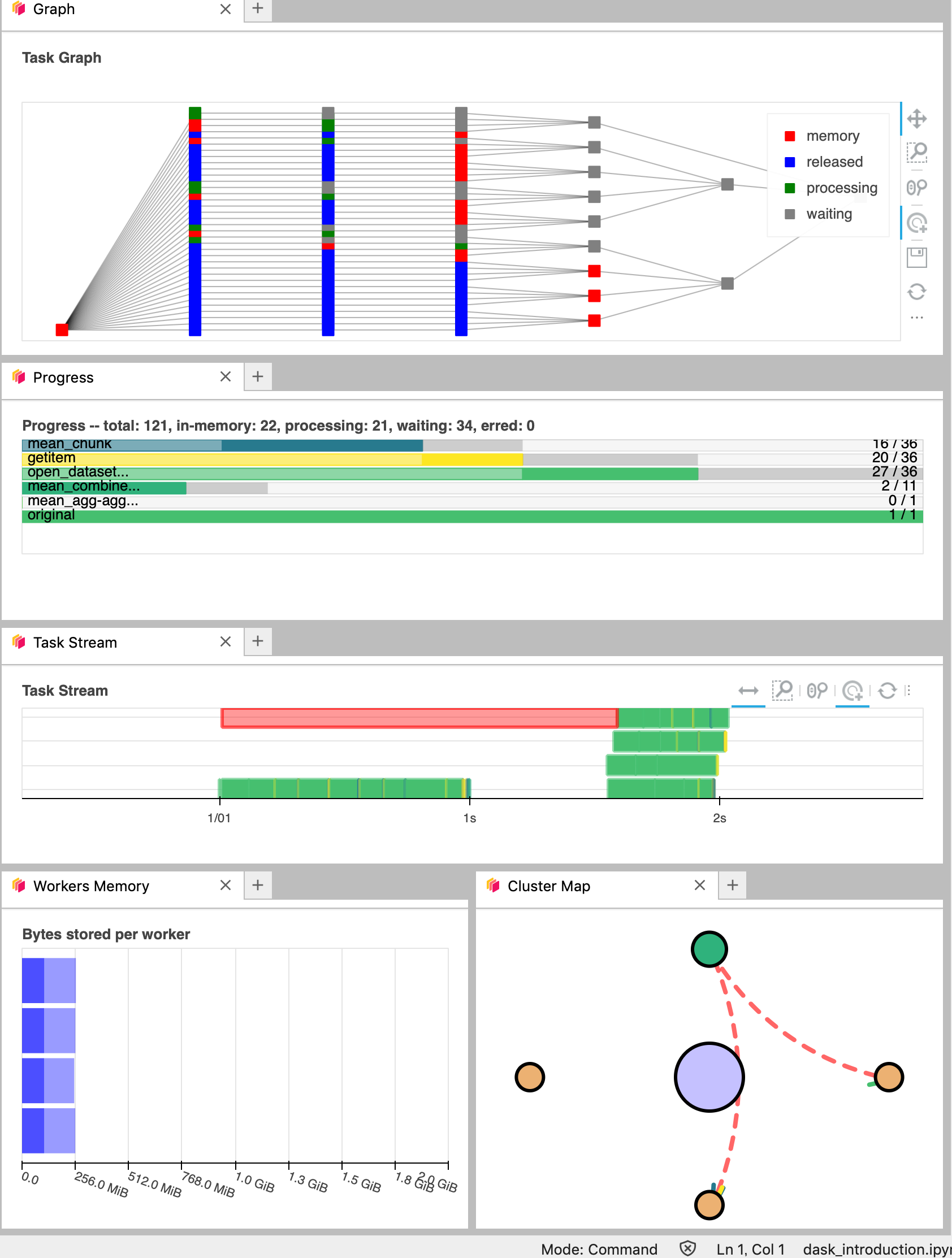
Calling compute() executes the graph and returns the selected result to the notebook. Watch the Dask Dashboard while this cell runs to see tasks move through the scheduler and workers.
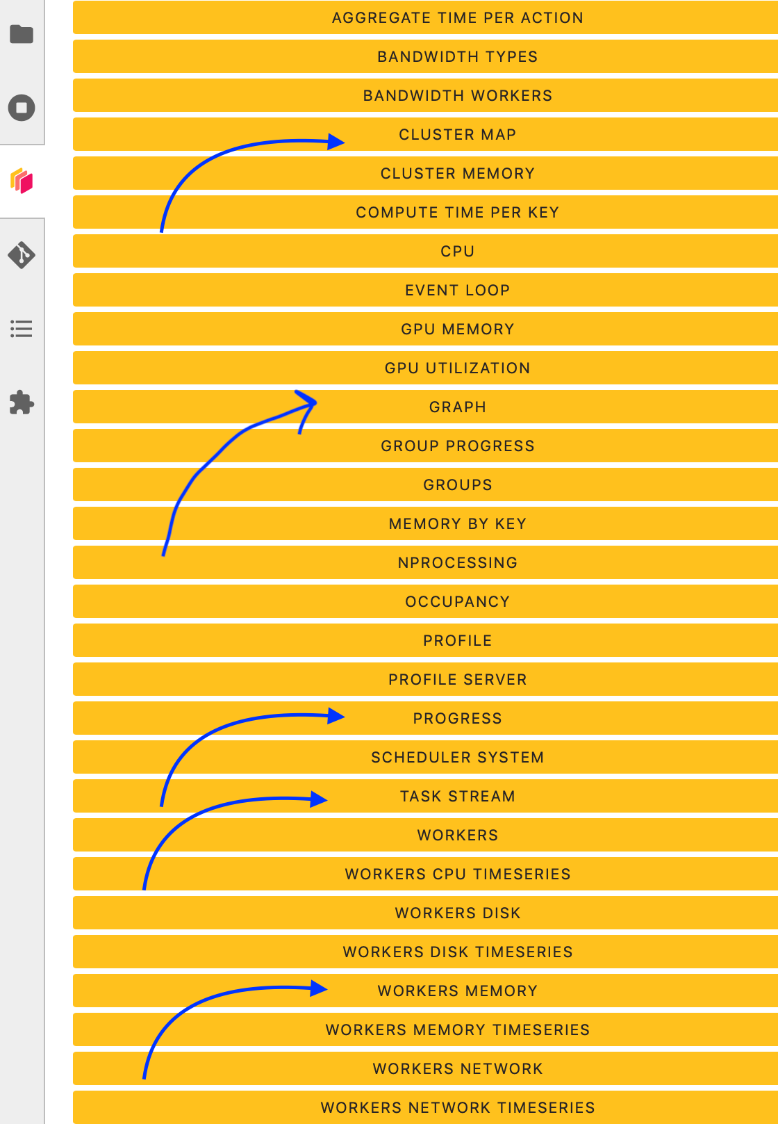
Use JupyterLab’s Dask sidebar to open panels such as Graph, Progress, Task Stream, and Workers Memory:
computed = plot_data.compute()
computed.plot(cmap="viridis")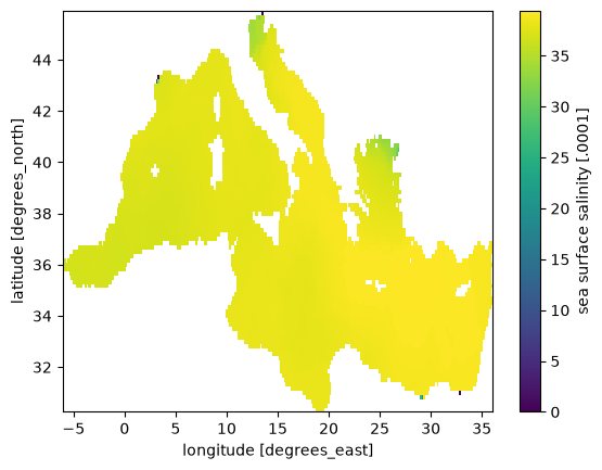
Close the Client
Close clients and clusters when you finish so their resources are available to other work.
client.close()