Accessing CDSE Data with the Pangeo Stack
import os
import numpy as np
import pandas as pd
import matplotlib.pyplot as plt
import cartopy.crs as ccrs
import cartopy.feature as cfeature
import pystac_client
import stackstac
import xarray as xr
from shapely.geometry import box
Start a cluster
# uncomment these lines to run dask gateway
# from dask.distributed import Client
# from dask_gateway import Gateway
# gateway = Gateway()
# cluster = gateway.new_cluster()
# cluster.scale(4)
# client = cluster.get_client()
# client
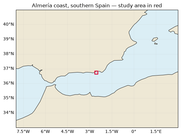
AOE: Almería coast, southern Spain
A smaller coastal box near Almería, chosen inside a single Sentinel-2 tile.
roi_bounds = (-2.65, 36.65, -2.45, 36.85)  # Almería coast: west, south, east, north

fig, ax = plt.subplots(figsize=(8, 5), subplot_kw={"projection": ccrs.PlateCarree()})
ax.set_extent([-8, 3, 33, 41])  # Zoom out for southern Spain and North Africa
ax.set_facecolor("#dbeef5")

ax.add_feature(cfeature.LAND.with_scale("50m"), facecolor="#eee8d5")
ax.coastlines("50m", linewidth=0.7)
ax.add_geometries([box(*roi_bounds)], ccrs.PlateCarree(), facecolor="none", edgecolor="crimson", linewidth=2)
ax.gridlines(draw_labels=["bottom", "left"], linewidth=0.4, alpha=0.3)
ax.set_title("Almería coast, southern Spain — study area in red");
S3 Credentials
taken from:
https://
In order to access the data from CloudFerro’s catalog, authentication is required. To facilitate this, you will need to create an account in the Copernicus Data Space Ecosystem (CDSE). The registration process is quick and can be completed in under 60 seconds. You can find the registration link here: https://
Once you have created an account, the same URL will redirect you to the section where you can generate your S3 Credentials. To do this, simply click the Add Credential button. This will allow you to define an expiration date for your credentials.
After selecting the expiration date, you will have successfully created your own S3 credentials. Please make sure to save the secret key at this point, as it will not be displayed again.
Now that you have your S3 credentials, you can use them to connect to the STAC catalog. By utilizing the os package, you will set environment variables to authenticate yourself as a valid user for the S3 protocol.
The only variables you need to configure are:
CDSE_S3_ACCESS_KEYCDSE_S3_SECRET_KEY.
# os.environ["CDSE_S3_ACCESS_KEY"] = "CDSE_S3_ACCESS_KEY" # Replace with your keys!
# os.environ["CDSE_S3_SECRET_KEY"] = "CDSE_S3_SECRET_KEY" # Replace with your keys!

# or create a .env file with those two variables above and run this instead
with open(".env") as f:
    for line in f:
        key, value = line.strip().split("=", 1)
        os.environ[key] = value
os.environ["GDAL_HTTP_TCP_KEEPALIVE"] = "YES"
os.environ["AWS_S3_ENDPOINT"] = "eodata.dataspace.copernicus.eu"
os.environ["AWS_ACCESS_KEY_ID"] = os.environ.get("CDSE_S3_ACCESS_KEY")
os.environ["AWS_SECRET_ACCESS_KEY"] = os.environ.get("CDSE_S3_SECRET_KEY")
os.environ["AWS_HTTPS"] = "YES"
os.environ["AWS_VIRTUAL_HOSTING"] = "FALSE"
os.environ["GDAL_HTTP_UNSAFESSL"] = "YES"
# Dask Gateway workers need these settings too (run after creating client).
# if "client" in globals():
# cdse_env = {key: os.environ[key] for key in ["AWS_ACCESS_KEY_ID", "AWS_SECRET_ACCESS_KEY", "AWS_S3_ENDPOINT", "AWS_HTTPS", "AWS_VIRTUAL_HOSTING"]}
# client.register_worker_callbacks(setup=lambda: os.environ.update(cdse_env))
Connecting to the STAC Catalog
We connect to the Copernicus STAC catalog, available at the endpoint: https://
URL = "https://stac.dataspace.copernicus.eu/v1"
cat = pystac_client.Client.open(URL)
Open the daily cube for this area
daily_surface_cube = xr.open_zarr(
    "https://s3.waw4-1.cloudferro.com/EarthCODE/OSCAssets/med_cubes/ocean-med-daily-surface-cube.zarr",
    group="0", chunks={}, consolidated=True, decode_coords="all",
)

surface_region = daily_surface_cube.sel(
    lon=slice(roi_bounds[0], roi_bounds[2]),
    lat=slice(roi_bounds[1], roi_bounds[3]),
)

daily_surface_cubeparams = {
"max_items": 12,
"collections": "sentinel-2-l2a",
"datetime": "2017-06-01/2017-12-31",
"bbox": roi_bounds,
"query": {"eo:cloud_cover": {"lte": 20}},
"sortby": "properties.eo:cloud_cover", # Least cloudy scenes first
}
Select six scenes
Take the six least cloudy scenes for this smaller box in July–August 2017.
items = list(cat.search(**params).items_as_dicts())
Creating DataCube from STAC
After performing the search, we can create a STACK object from the obtained items. In the definition of the STACK object, the following parameters must be declared:
items: The STAC items that will be included in the stack object.resolution: The desired output resolution.bounds_latlon: The spatial bounding box of the output, given in degrees of latitude and longitude.chunksize: The chunk size to be used for the Dask array.epsg: The EPSG code for the coordinate reference system to which the data will be reprojected.gdal_env: GDAL configuration options to be used when opening and reading the datasets.
note: added a workaround for compatibility reasons
# Temporary compatibility wrappers for stackstac 0.5.0 / NumPy 2 / pandas 3.
from unittest.mock import patch

_can_cast, _to_datetime = np.can_cast, pd.to_datetime
with (
    patch(
        "numpy.can_cast",
        lambda from_, to, casting="safe": _can_cast(np.result_type(from_), to, casting),
    ),
    patch(
        "pandas.to_datetime",
        lambda *args, infer_datetime_format=None, **kwargs: _to_datetime(*args, **kwargs),
    ),
):
    stack = stackstac.stack(
        items=items,
        sortby_date=False,  # Keep least-cloudy scenes first
        rescale=False,  # Raw DN: 0 is nodata; apply the N0500 offset below
        assets=["B04_20m", "B03_20m", "B02_20m", "B05_20m"],  # RGB + red edge for NDCI
        resolution=1 / 1200,  # Small-area RGB preview (degrees)
        bounds_latlon=roi_bounds,
        chunksize=512,
        xy_coords="center",
        epsg=4326,
        gdal_env=stackstac.DEFAULT_GDAL_ENV.updated(
            {
                "GDAL_NUM_THREADS": -1,
                "GDAL_HTTP_UNSAFESSL": "YES",
                "GDAL_HTTP_TCP_KEEPALIVE": "YES",
                "AWS_VIRTUAL_HOSTING": "FALSE",
                "AWS_HTTPS": "YES",
            }
        ),
    )

stack = stack.where(stack > 0)  # Mask no-data pixels
stack = stack.sortby("time").compute()
rgb = stack.sel(band=["B04_20m", "B03_20m", "B02_20m"])
rgb.plot.imshow(rgb="band", col="time", col_wrap=3, robust=True, size=3)
<xarray.plot.facetgrid.FacetGrid at 0x1774e52b0>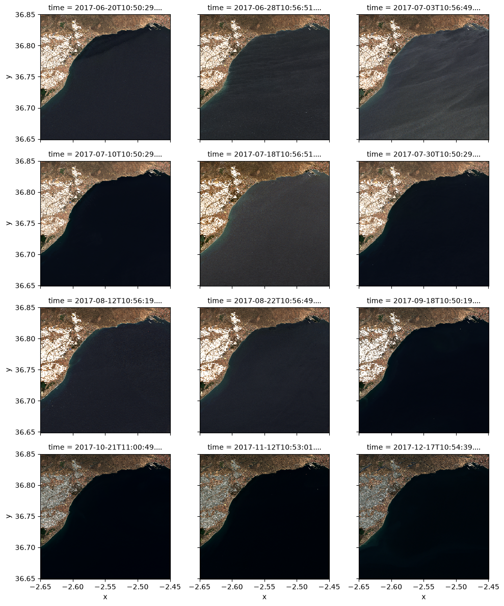
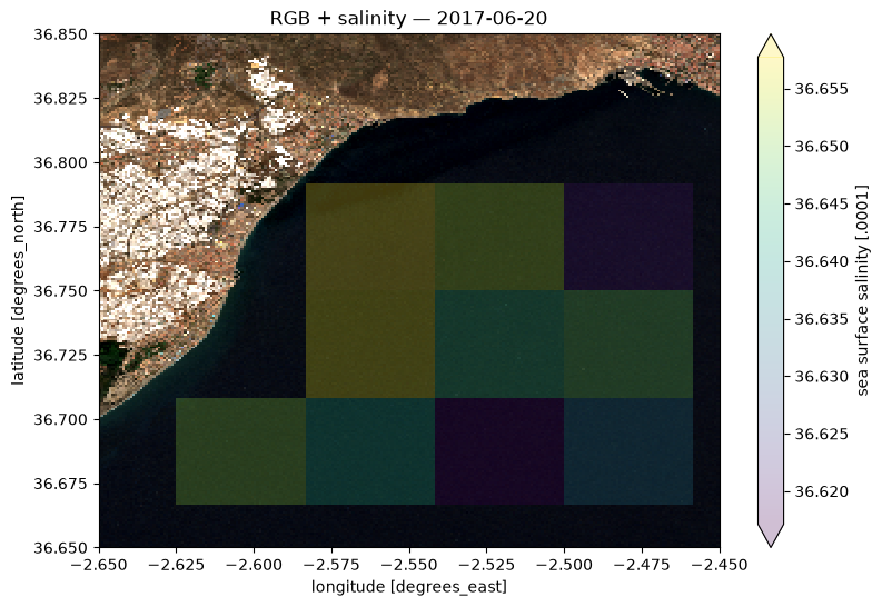
Overlay the first displayed date and salinity
selected_day = str(stack.time.values[0])[:10]
ax = rgb.isel(time=0).plot.imshow(rgb="band", robust=True, figsize=(9, 6)).axes
surface_region.sos.sel(time=selected_day).plot(ax=ax, cmap="viridis", alpha=0.25, robust=True)
ax.set(xlim=(roi_bounds[0], roi_bounds[2]), ylim=(roi_bounds[1], roi_bounds[3]), title=f"RGB + salinity — {selected_day}");
Compare NDCI and salinity over time
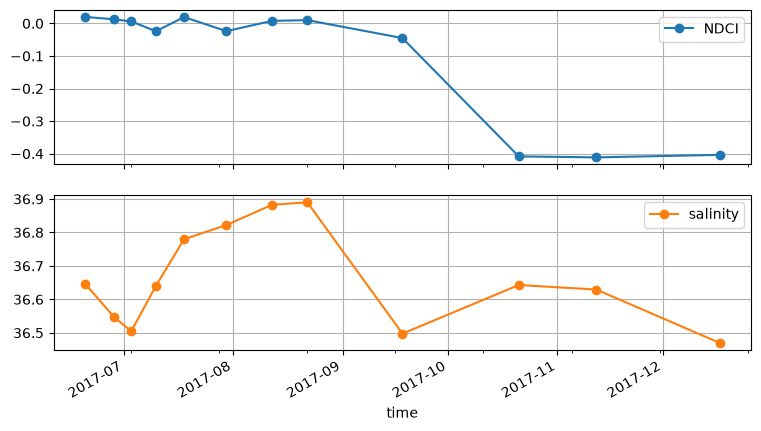
NDCI (Normalized Difference Chlorophyll Index) uses red-edge and red reflectance:
NDCI = (B05 - B04) / (B05 + B04)
Compare its daily mean with salinity (sos) over the same ocean pixels. NDCI is a relative chlorophyll-sensitive index, not chlorophyll concentration; it was developed for productive, turbid coastal waters and is less informative in clear, low-chlorophyll water (original paper).
bands = stack.assign_coords(time=stack.time.dt.floor("D")) - 1000  # N0500 offset; scale cancels
bands = bands.where(bands >= 0)  # Exclude negative reflectance and no-data pixels
red, red_edge = bands.sel(band="B04_20m", drop=True), bands.sel(band="B05_20m", drop=True)
ndci = (red_edge - red) / (red_edge + red).where(red_edge + red > 0)
ndci
salinity = surface_region.sos.sel(time=bands.time).interp(lon=bands.x, lat=bands.y, method="nearest")
water = xr.Dataset({"NDCI": ndci, "salinity": salinity}).where(ndci.notnull() & salinity.notnull())
waterseries = water.mean(("x", "y")).compute().to_dataframe()[["NDCI", "salinity"]]
series
series.plot(subplots=True, marker="o", figsize=(9, 5), grid=True); # Separate scales, shared dates
Network request benchmark
Computing close to the data can make downloads much faster.
Close to the data on the cloud
Running on a small machine with 2 GB RAM near the data storage:
| Source | Downloaded | Wall time | Total CPU time |
|---|---|---|---|
| CDSE Sentinel-2 | 117 MiB | 1.96 s | 570 ms |
| EarthCODE cube (CloudFerro) | 102 MiB | 1.21 s | 449 ms |
Running locally
Running the same benchmark locally over a reasonably fast internet connection:
| Source | Wall time | Total CPU time |
|---|---|---|
| CDSE Sentinel-2 | 11.2 s | 598 ms |
| EarthCODE cube (CloudFerro) | 12.1 s | 578 ms |
In this run, downloading close to the data was approximately 6× faster for CDSE and 10× faster for the cube.
Wall time is the elapsed time you wait. CPU time measures processor work, excluding time spent waiting for the network.
# %%time

# import s3fs
# cdse_s3 = s3fs.S3FileSystem(endpoint_url="https://eodata.dataspace.copernicus.eu")  # Uses the AWS credentials set above
# cube_s3 = s3fs.S3FileSystem(anon=True, endpoint_url="https://s3.waw4-1.cloudferro.com")

# cdse_bytes, i = 0, 0
# while cdse_bytes < 100 * 1024**2:
#     cdse_bytes += len(cdse_s3.cat_file(items[i % len(items)]["assets"]["B04_20m"]["href"]))
#     i += 1
# cdse_bytes / 1024**2
- Mishra, S., & Mishra, D. R. (2012). Normalized difference chlorophyll index: A novel model for remote estimation of chlorophyll-a concentration in turbid productive waters. Remote Sensing of Environment, 117, 394–406. 10.1016/j.rse.2011.10.016