Dask 101

Context¶

We will be using Dask with Xarray to parallelize our data analysis. The analysis is very similar to what we have done in previous examples, but this time we will use data with global coverage that we read from the SeasFire Cube.

We will use a local Dask distributed client from the agile26-pangeo conda environment.

Data¶

In this workshop, we will be using the SeasFire Data Cube available through the EarthCODE Open Science Catalog.

Alonso, Lazaro, Gans, Fabian, Karasante, Ilektra, Ahuja, Akanksha, Prapas, Ioannis, Kondylatos, Spyros, Papoutsis, Ioannis, Panagiotou, Eleannna, Michail, Dimitrios, Cremer, Felix, Weber, Ulrich, & Carvalhais, Nuno. (2022). SeasFire Cube: A Global Dataset for Seasonal Fire Modeling in the Earth System (0.4) [Data set]. Zenodo. Alonso et al. (2024). The same dataset can also be downloaded from Zenodo: https://zenodo.org/records/13834057

import dask.distributed
import xarray

Parallelize with Dask¶

We know from previous chapter cloud native formats 101 that chunking is key for analyzing large datasets. In this episode, we will learn to parallelize our data analysis using Dask on our chunked dataset.

What is Dask ?¶

Dask scales the existing Python ecosystem: with very or no changes in your code, you can speed-up computation using Dask or process bigger than memory datasets.

Dask is a flexible library for parallel computing in Python.
It is widely used for handling large and complex Earth Science datasets and speed up science.
Dask is powerful, scalable and flexible. It is the leading platform today for data analytics at scale.
It scales natively to clusters, cloud, HPC and bridges prototyping up to production.
The strength of Dask is that is scales and accelerates the existing Python ecosystem e.g. Numpy, Pandas and Scikit-learn with few effort from end-users.

It is interesting to note that at first, Dask has been created to handle data that is larger than memory, on a single computer. It then was extended with Distributed to compute data in parallel over clusters of computers.

How does Dask scale and accelerate your data analysis?¶

Dask proposes different abstractions to distribute your computation. In this Dask Introduction section, we will focus on Dask Array which is widely used in pangeo ecosystem as a back end of Xarray.

As shown in the previous section Dask Array is based on chunks. Chunks of a Dask Array are well-known Numpy arrays. By transforming our big datasets to Dask Array, making use of chunk, a large array is handled as many smaller Numpy ones and we can compute each of these chunks independently.

How does Xarray with Dask distribute data analysis?¶

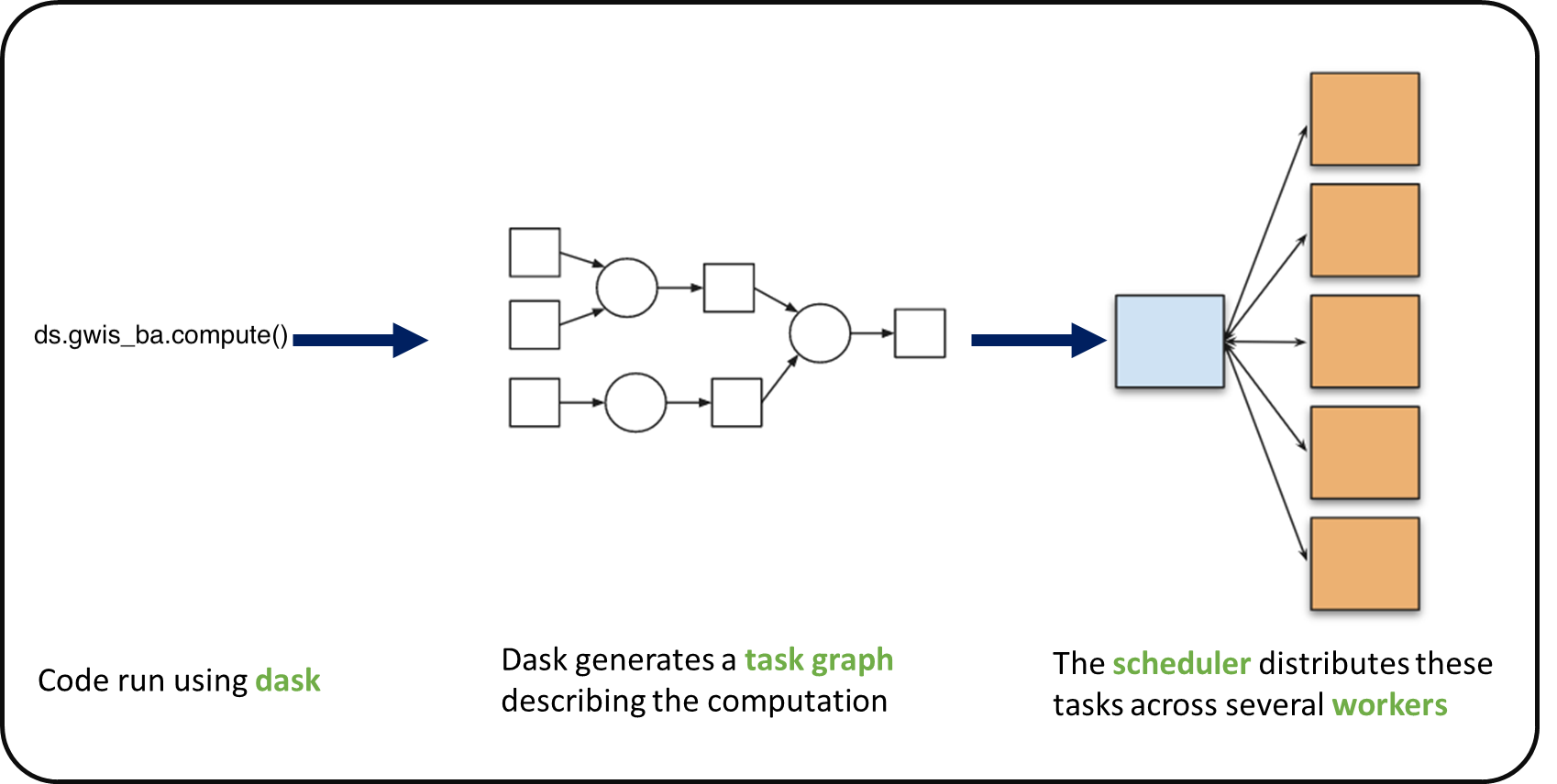
When we use chunks with Xarray, the real computation is only done when needed or asked for, usually when invoking compute() or load() functions. Dask generates a task graph describing the computations to be done. When using Dask Distributed a Scheduler distributes these tasks across several Workers.

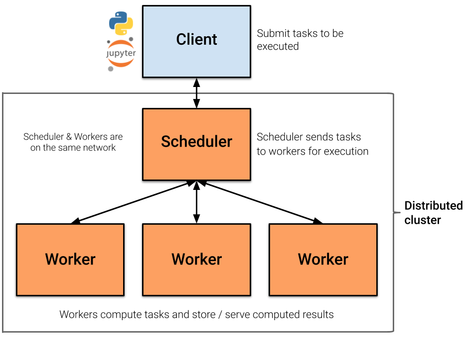
What is a Dask Distributed cluster ?¶

A Dask Distributed cluster is made of two main components:

a Scheduler, responsible for handling computations graph and distributing tasks to Workers.
One or several (up to 1000s) Workers, computing individual tasks and storing results and data into distributed memory (RAM and/or worker’s local disk).

A user usually needs Client and Cluster objects as shown below to use Dask Distributed.

Where can we deploy a Dask distributed cluster?¶

Dask distributed clusters can be deployed on your laptop or on distributed infrastructures such as cloud, HPC centres, and Hadoop. A Dask distributed Cluster object is responsible for deploying and scaling a Dask cluster on the underlying resources.

For this workshop, we use a local Dask distributed cluster created from the notebook session.

Dask distributed Client¶

The Dask distributed Client is what allows you to interact with Dask distributed clusters. When using Dask distributed, you always need to create a Client object. Once a Client has been created, it will be used by default by each call to a Dask API, even if you do not explicitly use it.

No matter the Dask API (e.g. Arrays, Dataframes, Delayed, Futures, etc.) that you use, under the hood, Dask will create a Directed Acyclic Graph (DAG) of tasks by analysing the code. Client will be responsible for submitting this DAG to the Scheduler along with the final result you want to compute. The Client will also gather results from the Workers and aggregate it back in its underlying Python process.

Using Client() with no argument creates a local Dask cluster with a number of workers and threads based on the resources available to this notebook session.

from dask.distributed import Client

client = Client()   # create a local dask cluster on the local machine.
client

/opt/miniconda3/envs/pangeo/lib/python3.13/site-packages/distributed/node.py:187: UserWarning: Port 8787 is already in use.
Perhaps you already have a cluster running?
Hosting the HTTP server on port 50652 instead
  warnings.warn(

Inspecting the Cluster Info section above gives us information about the created cluster: we have 2 or 4 workers and the same number of threads (e.g. 1 thread per worker).

# close client to clean resources
# Note, you can run this tutorial locally if you uncomment this line 
client.close()

Scaling Your Computation Locally¶

The local Dask cluster created above is enough for this workshop. It lets Xarray process chunked arrays lazily and schedule work across local worker processes.

On larger infrastructures, Dask can also connect to managed clusters, but those deployments are outside the scope of this local AGILE 2026 workshop.

# Reuse the local client created above.
client

Local Cluster Resources¶

The default local cluster uses the CPU and memory available to your notebook session. Keep the default settings unless an instructor asks you to adjust them.

client.cluster

# Optional: request a small number of local workers.
# Adjust this only if your laptop has enough CPU and memory.
# client.cluster.scale(2)
client.cluster

Use the Local Client¶

The Client created earlier remains the default scheduler for the Dask-backed Xarray computations below.

client

Dask Dashboard¶

Dask provides a dashboard for inspecting task graphs, workers, memory use, and progress. The dashboard link is available from the local client:

client.dashboard_link

If the Dask JupyterLab extension is available in your environment, you can also open dashboard panes directly inside JupyterLab. The dashboard is useful for understanding when computations are lazy, when they trigger execution, and how work is distributed across local workers.

Dask Distributed computations on our dataset¶

Let’s open the SeasFire dataset we previously looked at, select a single location over time, visualize the task graph generated by Dask, and observe the Dask Dashboard.

http_url = "https://s3.waw4-1.cloudferro.com/EarthCODE/OSCAssets/seasfire/seasfire_v0.4.zarr/"

ds = xarray.open_dataset(
	http_url,
	engine='zarr',
    chunks={},
	consolidated=True
)
ds

mask= ds['lsm'][:,:]
gwis_all= ds.gwis_ba.resample(time="1YE").sum()
gwis_all= gwis_all.where(mask>0.5)

gwis_2020= gwis_all.sel(time='2020-08-01', method='nearest')
gwis_2020.data

gwis_2020.data.visualize(optimize_graph=True)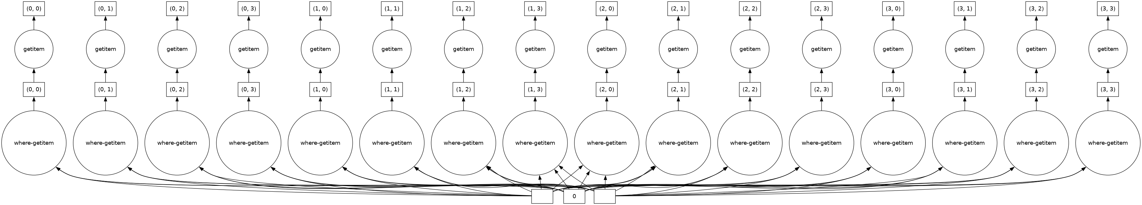

Did you notice something on the Dask Dashboard when running the two previous cells?

We didn’t ‘compute’ anything. We just built a Dask task graph with it’s size indicated as count above, but did not ask Dask to return a result.

Note that underneath, dask optimizes the execution graph (opaquely), so as to minimize overheads and overall execution resources (hence why we’re passing optimize_graph=True)

Computing¶

Calling compute on our Xarray object will trigger the execution on the Dask Cluster. Alternatively any action that would demand the computation of our data (e.g. plotting) would trigger the execution of our workflow.

You should be able to see how Dask is working on Dask Dashboard.

gwis_2020.plot()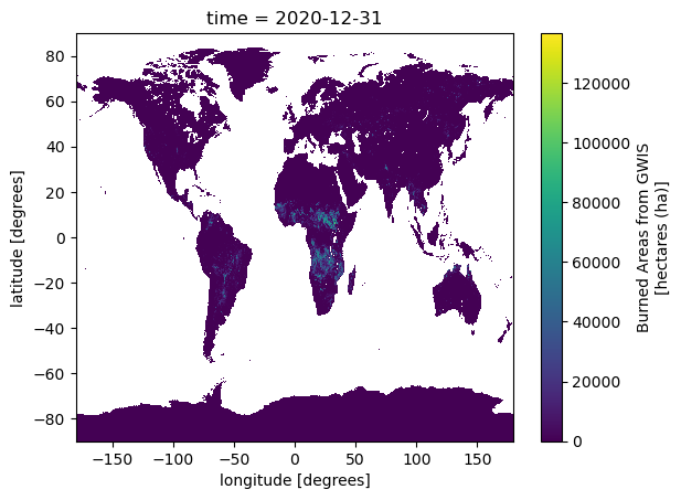

Closing Clusters¶

Close Clusters to Clean Resources for the next exercise (generally a good practice!)

# close client to clean resources
client.close()

References¶

Alonso, L., Gans, F., Karasante, I., Ahuja, A., Prapas, I., Kondylatos, S., Papoutsis, I., Panagiotou, E., Mihail, D., Cremer, F., Weber, U., & Carvalhais, N. (2024). SeasFire Cube: A Global Dataset for Seasonal Fire Modeling in the Earth System. Zenodo. 10.5281/ZENODO.13834057