Xarray 101 - EarthCODE Tutorials

from pystac.extensions.storage import StorageExtension
from datetime import datetime
from pystac_client import Client as pystac_client
from odc.stac import configure_rio, stac_load
import matplotlib.pyplot as plt

import xarray

What is xarray?¶

Xarray introduces labels in the form of dimensions, coordinates and attributes on top of raw NumPy-like multi-dimensional arrays, which allows for a more intuitive, more concise, and less error-prone developer experience.

How is xarray structured?¶

Xarray has two core data structures, which build upon and extend the core strengths of NumPy and Pandas libraries. Both data structures are fundamentally N-dimensional:

DataArray is the implementation of a labeled, N-dimensional array. It is an N-D generalization of a Pandas.Series. The name DataArray itself is borrowed from Fernando Perez’s datarray project, which prototyped a similar data structure.
Dataset is a multi-dimensional, in-memory array database. It is a dict-like container of DataArray objects aligned along any number of shared dimensions, and serves a similar purpose in xarray as the pandas.DataFrame.

Data can be read from online sources, as in the example below where we loaded metadata

http_url = "https://s3.waw4-1.cloudferro.com/EarthCODE/OSCAssets/seasfire/seasfire_v0.4.zarr/"

ds = xarray.open_dataset(
	http_url,
	engine='zarr',
    chunks={},
	consolidated=True
	# storage_options = {'token': 'anon'}
)
ds

Accessing Coordinates and Data Variables¶

DataArray, within Datasets, can be accessed through:

the dot notation like Dataset.NameofVariable
or using square brackets, like Dataset[‘NameofVariable’] (NameofVariable needs to be a string so use quotes or double quotes)

ds.latitude

ds.lai

ds[‘lai’] is a one-dimensional xarray.DataArray with dates of type datetime64[ns]

ds['lai']

ds['lai'].attrs

{'aggregation': 'Temporal | mean',
 'creator_notes': 'Seasonality in Nan values for high latitudes, due to seasonality in the data availability',
 'description': 'The MCD15A2H Version 6 Moderate Resolution Imaging Spectroradiometer (MODIS) Level 4, Combined Fraction of Photosynthetically Active Radiation (FPAR), and Leaf Area Index (LAI) product is an 8-day composite dataset with 500 meter pixel size. The algorithm chooses the best pixel available from all the acquisitions of both MODIS sensors located on NASA’s Terra and Aqua satellites from within the 8-day period.LAI is defined as the one-sided green leaf area per unit ground area in broadleaf canopies and as one-half the total needle surface area per unit ground area in coniferous canopies. FPAR is defined as the fraction of incident photosynthetically active radiation (400-700 nm) absorbed by the green elements of a vegetation canopy.',
 'downloaded_from': 'https://lpdaac.usgs.gov/products/mcd15a2hv006/',
 'long_name': 'Leaf Area Index ',
 'provider': 'NASA',
 'units': 'm²/m²'}

Xarray and Memory usage¶

Once a Data Array|Set is opened, xarray loads into memory only the coordinates and all the metadata needed to describe it. The underlying data, the component written into the datastore, are loaded into memory as a NumPy array, only once directly accessed; once in there, it will be kept to avoid re-readings. This brings the fact that it is good practice to have a look to the size of the data before accessing it. A classical mistake is to try loading arrays bigger than the memory with the obvious result of killing a notebook Kernel or Python process. If the dataset does not fit in the available memory, then the only option will be to load it through the chunking; later on, in the tutorial ‘chunking_introduction’, we will introduce this concept.

As the size of the data is not too big here, we can continue without any problem. But let’s first have a look to the actual size and then how it impacts the memory once loaded into it.

import numpy as np

print(f'{np.round(ds.lai.nbytes / 1024**3, 2)} GB') # all the data are automatically loaded into memory as NumpyArray once they are accessed.

3.73 GB

ds.lai.data

As other datasets have dimensions named according to the more common triad lat,lon,time a renomination is needed.

Selection methods¶

As underneath DataArrays are Numpy Array objects (that implement the standard Python x[obj] (x: array, obj: int,slice) syntax). Their data can be accessed through the same approach of numpy indexing.

ds.lai[0,100,100].load()

As it is not easy to remember the order of dimensions, Xarray really helps by making it possible to select the position using names:

.isel -> selection based on positional index
.sel -> selection based on coordinate values

ds.lai.isel(time=0, latitude=100, longitude=100)

The more common way to select a point is through the labeled coordinate using the .sel method.

Time is easy to be used as there is a 1 to 1 correspondence with values in the index, float values are not that easy to be used and a small discrepancy can make a big difference in terms of results.

Coordinates are always affected by precision issues; the best option to quickly get a point over the coordinates is to set the sampling method (method=‘’) that will search for the closest point according to the specified one.

Options for the method are:

pad / ffill: propagate last valid index value forward
backfill / bfill: propagate next valid index value backward
nearest: use nearest valid index value

Another important parameter that can be set is the tolerance that specifies the distance between the requested and the target (so that abs(index[indexer] - target) <= tolerance) from documentation.

ds.lai.sel(time=datetime(2020, 1, 8), method='nearest')

ds.lai.sel(latitude=46.3, longitude=8.8, method='nearest').isel(time=0)

ds.lai.isel(longitude=100).longitude.values.item()

-154.875

Plotting¶

Plotting data can easily be obtained through matplotlib.pyplot back-end matplotlib documentation.

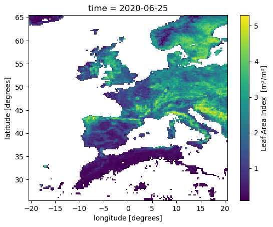
As the exercise is focused on an Area Of Interest, this can be obtained through a bounding box defined with slices.

Plot fires

lai_aoi = ds.lai.sel(latitude=slice(65.5,25.5), longitude=slice(-20.5,20.5))
lai_aoi.sel(time=datetime(2020,6,23), method='nearest').plot()

Basic Maths and Stats¶

# E.g. example scaling 

lai_aoi * 0.0001 + 1500

Statistics and Aggregation¶

Calculate simple statistics:

lai_aoi.min()
lai_aoi.max()
lai_aoi.mean()

Aggregate by month if the dataset spans multiple months:

lai_monthly = lai_aoi.groupby(lai_aoi.time.dt.month).mean()
lai_monthly

Masking¶

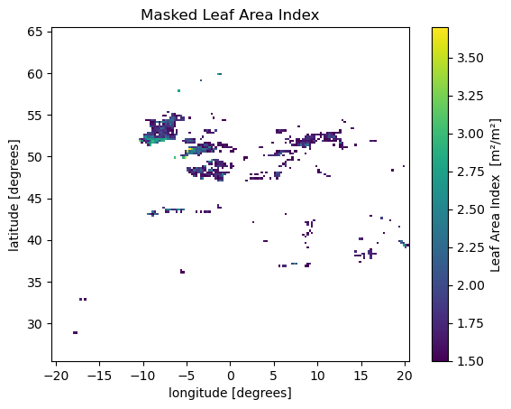
Not all values are valid and masking all those which are not in the valid range is necessary. Masking can be achieved through the method DataSet|Array.where(cond, other) or xr.where(cond, x, y).

The difference consists in the possibility to specify the value in case the condition is positive or not; DataSet|Array.where(cond, other) only offer the possibility to define the false condition value (by default is set to np.NaN))


lai_masked = lai_aoi.where(lai_aoi >= 1.5) 
lai_masked

lai_masked.isel(time=0).plot(cmap='viridis')
plt.title("Masked Leaf Area Index")
plt.show()

mask = xarray.where((lai_aoi > 1.5), 1, 0)
mask.isel(time=0).plot()
plt.title("Masked Leaf Area Index")
plt.show()